Edited by Thom Ives

Find the Code on GitHub

Data is the new oil and new gold. Sorta. There is a lot of hype around data science. It is essential, or at least very helpful, to have a good foundation in statistical principles before diving into this field.

Data can tell us amazing stories if we ask it the right questions. In order to ask the right questions, we need to ask some introductory questions, just like you might do when meeting a new person. Data is often characterized by the types of distributions that it contains. Knowing the kinds of distributions that each variable in your data fits is essential to determining what additional questions we should ask (i.e what further analyses we should perform to learn more).

When it comes to distributions of data, in the field of statistics or data science, the most common one is the normal distribution, and in this post, we will seek to thoroughly introduce it and understand it.

Contents

1. Introduction
2. History of The Normal Distribution
3. PDF and CDF of The Normal Distribution
4. Calculating the Probability of The Normal Distribution using Python
5. References

1. Introduction

A normal distribution (aka a Gaussian distribution) is a continuous probability distribution for real-valued variables. Whoa! That’s a tightly packed group of mathematical words. I understand! Trust me, it will make more sense as we explain it and use it. It is a symmetric distribution where most of the observations cluster around a central peak, which we call the mean. When collecting data, we expect to see this value more than any others when our data is normally distributed (i.e. this value will have the highest probability). Data values other than the mean will be less probable. The further the other values are from the mean the less probable they are. These other data values will taper off to lower and lower probabilities equally in both directions the farther they are from the mean value.

This distribution is very common in real world processes all around us. Many natural phenomena can be described very well with this distribution. The height of male students, the height of female students, IQ scores, etc. All of these and more follow a normal distribution. However, please keep in mind that data is NOT always normally distributed. Future posts will cover other types of probability distributions. We are going over the normal distribution first, because it is a very common and important distribution, and it is frequently used in many data science activities.

Let’s go a bit deeper into the mathematics used with the normal distribution. Although we are going deeper, I think the equations below will help you understand the normal distribution much better. More importantly, these additional mathematics will help you make better use of the normal distribution in your data science work.

2. History of the Normal Distribution

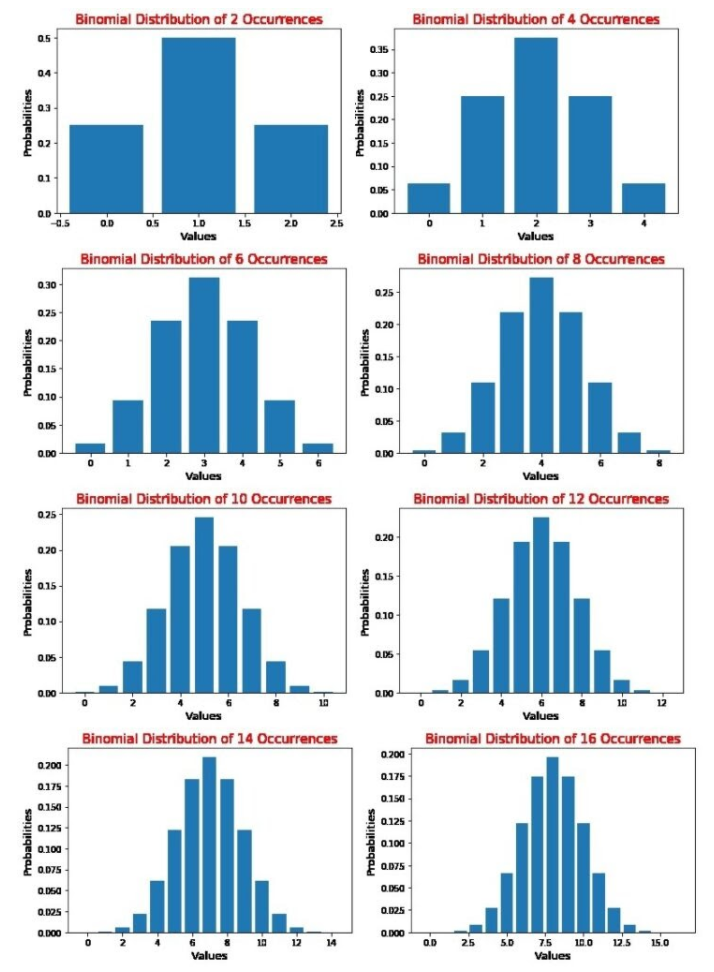
The discovery of the normal distribution was first attributed to Abraham de Moivre, as an approximation of a binomial distribution. Abraham de Moivre was an 18th CE French mathematician and was also a consultant to many gamblers. We know that the binomial distribution can be used to model questions such as “If a fair coin is tossed 200 times, what is the probability of getting more than 80 heads?” To know more about the binomial distribution, see this link. In order to solve such problems, de Moivre had to sum up all the probabilities of getting 81 heads, 82 heads up to 200 heads. In the process, he noticed that as the number of occurrences increased, the shape of the binomial distribution started becoming smooth.

Let us see how this is possible. We can plot the binomial distribution graphs of different occurrences of events using the following code, which is in the colab notebook named Calculating Probabilities using Normal Distributions in Python on the GitHub repo for this post.

Code Block 2.1

import scipy
from scipy.stats import binom 
import matplotlib.pyplot as plt 

# setting the values of n and p
n = 8
p = 0.5    # Here p = 0.5 as it is a binomial distribution with two outcomes(equal chances of success and failure)

# defining list of r values 
r_values = list(range(n + 1)) 

# list of pmf values 
dist = [binom.pmf(r, n, p) for r in r_values ] 

# plotting the graph  
plt.title(label="Binomial Distribution of  Occurrences", 
          fontsize=15, color="red")
plt.bar(r_values, dist)
plt.xlabel("Values", fontsize=13)
plt.ylabel("Probabilities", fontsize=13)
plt.show()

Here, when we use different values of n, we obtain the graphs shown below:

De Moivre hypothesized that if he could formulate an equation to model this curve, then such distributions could be better predicted. He introduced the concept of the normal distribution in the second edition of ‘The Doctrine of Chances‘ in 1738. Learn more on Abraham de Moivre here.

The normal distribution is very important because many of the phenomena in nature and measurements approximately follow the symmetric normal distribution curve.

One of the first applications of the normal distribution was to the analysis of errors of measurement made in astronomical observations, errors that occurred because of imperfect instruments and imperfect observers. Galileo in the 17th century noted that these errors were symmetric and that small errors occurred more frequently than large errors. This led to several hypothesized distributions of errors, but it was not until the early 19th century that it was discovered that these errors followed a normal distribution.

Online Stat Book

Enter Gauss and LaPlace

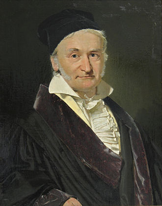
In 1823, Johann Carl Friedrich Gauss published Theoria combinationis observationum erroribus minimus obnoxiae, which is the theory of observable errors. In the third section of Theoria Motus, Gauss introduced the famous law of the normal distribution to analyze astronomical measurement data. Gauss made a series of general assumptions about observations and observable errors and supplemented them with a purely mathematical assumption. Then, in a very simple and elegant way, he was able to fit the curve of collected data from his experiments with an equation. The equation that reproduces the shape of this data was given the name ‘Gaussian Distribution’. The graph resembles a bell and is oftentimes called a bell-shaped curve.

Laplace (23 March 1749 – 5 March 1827) was the french mathematician who discovered the famous Central Limit Theorem (which we will be discussing more in a later post). He observed that, even if a population does not follow a normal distribution, as the number of the samples taken increases, the distribution of the sample means tends to be a normal distribution. (We saw an example of this in the case of a binomial distribution). So now, let us look deeply into all the equations these great mathematicians developed to fit the normal distribution and understand how they can be applied to real life situations.

3. PDF and CDF of The Normal Distribution

The probability density function (PDF) and cumulative distribution function (CDF) help us determine probabilities and ranges of probabilities when data follows a normal distribution. The CDF is the integration, from left to right, of the PDF. Using these two normal distribution functions, we can calculate different types of probability estimates from our normally distributed data.

3.1 : Probability Density Function (PDF)

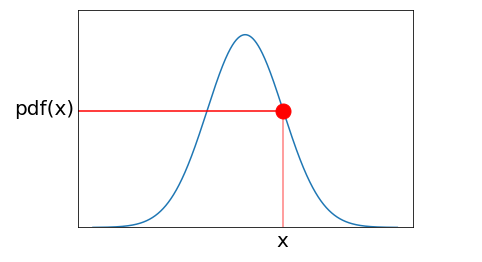
The probability density function (PDF) is a statistical expression that defines a probability distribution (the likelihood of an outcome) for a discrete random variable as opposed to a continuous random variable. When the PDF is graphically portrayed, the area under the curve will indicate the interval in which the variable will fall.

Investopedia

A continuous random variable X is said to follow the normal distribution if it’s probability density function (PDF) is given by:

\Large \tag*{Equation 3.1} f(x; \mu, σ) = \frac{1}{\sqrt{2 \pi \cdot \sigma^2}} \cdot e^{- \frac{1}{2} \cdot {\lparen \frac{x - \mu}{\sigma} \rparen}^2}

The variable µ is the mean of the data values. There are two types of means that we can use: 1) the population mean µ, and 2) the sample mean x̅. These are shown in equations 3.2. The population mean is the mean for ALL data for a specific variable. If you wanted to know the average height of 1^st graders in a specific elementary school, collecting the population mean is not a problem. However, it is NOT always possible to get all the values of a complete population (e.g. the height of all Ponderosa Pine trees in the world in the summer of 2020). When we cannot obtain the population mean, we must rely on the sample mean. How can we make sure that the sample mean is representative of the population mean? We will address this i greater detail in future posts. For now, it’s best to say that we want our sample to be as large and as unbiased as possible.

\tag*{Equation 3.2.a} \mu = \frac{1}{N}{\sum_{i=1}^N x_i} \tag*{Equation 3.2.b} \bar x = \frac{1}{n}{\sum_{i=1}^n x_i}

Once we have a mean value, we can also calculate σ, which is the standard deviation of our data from the mean value. I like to think of the standard deviation as the “average deviation” from the mean value of the data. The standard deviation is the way we communicate to each other how “spread out” the data is – how much it “deviates” from the mean value. Both µ and σ are called parameters of the normal distribution.

For the same reasons described above with the population and sample means, we sometimes have a standard deviation for the population σ, but oftentimes we must rely on a sample standard deviation s. Calculations for both of these standard deviations are shown in equations 3.3.

\tag*{Equation 3.3.a} σ=\sqrt{\frac{1}{N}\sum_{i=1}^N (x_i - \mu)^2} \tag*{Equation 3.3.b} s=\sqrt{\frac{1}{n-1}\sum_{i=1}^n (x_i - \bar x)^2}

Why do we divide sample variance by n-1 and not n?

The metrics of a population are called parameters and metrics of a sample are called statistics. The population variance is a parameter of the population and the sample variance is a statistic of the sample. The sample variance can be considered as an unbiased estimator of variance. What does unbiased mean?

In statistics, the bias (or bias function) of an estimator is the difference between this estimator’s expected value and the true value of the parameter being estimated. An estimator or decision rule with zero bias is called unbiased. In statistics, “bias” is an objective property of an estimator.

Wikipedia

If we are able to list out all possible samples of size n, from a population of size N, we will be able to calculate the sample variance of each sample. The sample variance will be an unbiased estimator of the population variance if the average of all sample variances is equal to the population variance.

We see that, in the sample variance, each observation is subtracted from the sample mean, which falls in the middle of the observations in the sample, whereas the population mean can be any value. So, the sample mean is just one possible position for the true population mean. And sometimes, the population mean can lie far away from the sample mean (depending on the current sampling).

The variance is the average of the sum of squares of the difference of the observations from the mean. So, when we use the sample mean as an approximation of the population mean for calculating the sample variance, the numerator (i.e. the sum of the squared distances from the mean) can be small at times. In those cases, we will get smaller sample variances. Hence, when we divide the sample variance by n, we underestimate (i.e get a biased value) the population variance. In order to compensate for this, we make the denominator of the sample variance n-1, to obtain a larger value. This reduces the bias of the sample variance as an estimator of the population variance.

So, when we divide the sample variances by n −1, the average of the sample variances for all possible samples is equal to the population variance. Thus we say that the sample variance will be an unbiased estimate of the population variance. Refer to this link for a detailed mathematical example of this theory.

Let’s understand the use case of the PDF with an example. Let’s assume that we are working with the heights of kids in the 1^st grade. We know from experience that such heights, when sampled in significant quantities, are normally distributed. However, we are in learning mode. Let’s not go out and actually measure the heights of 1^st graders. Let’s make some fake data that is normally distributed. How can we do that easily?

First, we need some reasonable numbers for µ and σ. Has someone already done data sampling work on the heights of 1^st graders? Yes! Check out THIS STUDY. The researchers of that study found µ = 37 inches and σ = 2 inches. Let’s use these parameters and some python code to create some fake data – a valuable skill to have when learning data science. We can create the PDF of a normal distribution using basic functions in Python. The rest of the code for this post is also in the colab notebook named Calculating Probabilities using Normal Distributions in Python in the GitHub repo developed for this post. The code blocks are in the post and the notebook are in the same order.

Code Block 3.1

import math

''' Probability Density Function (PDF) from Scratch '''
def PDF(x, mean, std_dev):
    probability = 1.0 / math.sqrt(2 * 3.141592*(std_dev)**2)  # first part of equation
    probability *= math.exp(-0.5 * ((x - mean)/std_dev)**2)  # multiply first part to second part


    return probability

X = []

''' Create Fake Normally Distributed Data with Mean of 37, and Std_Dev of 2 '''
for x in range(29, 46):
    y = PDF(x, 37, 2)
    
    ''' We want to create fake data by replicating x according to it's probability '''
    N_vals_at_y = int(round(y * 1001, 0))
    for i in range(N_vals_at_y):
      X.append(x)


# Finding mean
mean = round(sum(X)/len(X), 4)


# Finding Standard Deviation
std_dev = 0.0
N = len(X)
for x in X:
  std_dev += (x - mean)**2

std_dev /= N
std_dev = math.sqrt(std_dev)
std_dev = round(std_dev, 2)

print(f'We fake measured the heights of {N} 1st graders.')
print(f’The mean is {mean}’)
print(f’The standard deviation is {std_dev}’)

The output from the above block is

We fake measured the heights of 1000 1st graders.
The mean is 37.0
The standard deviation is 1.99

So, now we have created our PDF function from scratch without using any modules like NumPy or SciPy. We can get the PDF of a particular value by using the next block of code from our notebook:

Code Block 3.2

x = 39
print(PDF(x, 37, 2))

Here, we find the PDF value corresponding to x= 39. The output of the above block is:

0.12098537484471858

We can also generate a PDF of a normal distribution using the python modules NumPy, SciPy, and visualize them with Matplotlib. Before that, let’s understand the functionalities of each of these modules. 

NumPy is a Python package that stands for ‘Numerical Python’. This library is mainly used for scientific computing, and it contains powerful n-dimensional array objects and other powerful data structures (e.g. it implements multi-dimensional arrays and matrices). SciPy is an open-source Python library and is very helpful in solving scientific and mathematical problems. It is built on NumPy and allows the user to manipulate and visualize data. Matplotlib is an amazingly good and flexible plotting and visualization library in Python. Matplotlib is also built on NumPy. Matplotlib provides several plots such as line, bar, scatter, histogram, and more.

We can generate the PDF of the normal distribution and visualizations of it using these modules. We start with the function norm.pdf(x, loc, scale), where, loc is the variable that specifies the mean and scale specifies the standard deviation. For more details on the function, click here.

Code Block 3.3

import scipy
import numpy as np
import matplotlib.pyplot as plt 
from scipy.stats import norm

figure,ax = plt.subplots()
 
X = []
Y = []
 
for x in np.arange(29, 46, 0.1):
    X.append(x)
    y = norm.pdf(x=x, loc=37.0, scale=2)
    Y.append(y)

ax.set_xlabel('1st Grader Heights')
ax.set_ylabel('Probabilities of 1st Grader Heights')
ax.set_title('PDF of 1st Grader Heights, mu = 37, sigma = 2')
plt.plot(X, Y)
plt.show()

The output of the code above yields the plot shown in figure 3.1.

The heights of the kids are stored as elements x inside the vector X. If we want the probability for a specific height x = 39″, we only need to enter that specific value of x into the norm.pdf method call as shown in the code lines below, which can be added to the end of the code lines above.

Code Block 3.4

x = 39
p = norm.pdf(x=x, loc=37.0, scale=2)
print(f'The probability of a 1st grader being "{x}" is {p}.')

The python code should run from a command console or a notebook. Adding the above lines to the end of the previous code block the output will be:

The probability of a 1st grader being 39" is 0.12098536225957168.

We can see that the output of the PDF function that we created from scratch, as well as the one using the Python modules, return the same value 0.12098536225957168. Please realize that 39″ is like a bucket of all students that are between 39.0″ and 39.99__”. This may not be clear now, but when we start to use the cumulative distribution function below, it will become more clear.

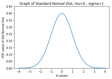
3.2 : Standard Normal Distribution

The scales used to measure variables do not necessarily represent the importance of the different variables in our studies and may end up creating a bias in our thinking compared to other variables. For example, one variable in our data may have very large numbers, and other variables may have much smaller numbers. We don’t want those larger numbers to unduly influence the training of models or to unduly influence our interpretation of the importance of one variable over others. Also, if the data is too widely spread out, outliers become more likely and can negatively affect model parameters during training. Thus, we frequently standardize data. We can standardize data in two steps:  1) subtract the mean from each of the values of the sample and then divide those differences by the standard deviation [(X – µ)/σ]. This process is called data normalization, and when we do this we transform a  normal distribution into what we call a standard normal distribution.

After performing the above mathematical standardization operations, the standard normal distribution will have µ = 0 and σ = 1. In summary, we can transform all the observations of any normal random variable X with mean μ and variance σ to a new set of observations of another normal random variable Z with µ = 0 and σ = 1. The PDF of the standard normal distribution is given by equation 3.4.

\tag*{Equation 3.4} f(z)=\frac{1}{2\pi}exp(\frac{-z^2}{2})

What is an example use-case where we’d want to use a standard normal distribution? Consider again the heights of 1^st grade students. Suppose that you’ve expanded the scope of your study. Perhaps now, due to the breadth of source data, the data is more widely spread out, and / or the data may be measured in different scales (i.e. centimetres or inches). We would want to normalize such data.

We can find the PDF of a standard normal distribution using basic code by simply substituting the values of the mean and the standard deviation to 0 and 1, respectively, in the first block of code.

Also, since norm.pdf() returns a PDF value, we can use this function to plot the standard normal distribution function with a mean = 0 and a standard deviation = 1, respectively. We graph this standard normal distribution using SciPy, NumPy and Matplotlib. We use the domain of −4 < 𝑥 < 4 for visualization purposes (4 standard deviations away from the mean on each side) to ensure that both tails become close to 0 in probability. With the values of 𝜇 = 0 and 𝜎 = 1, the code block below produces the plot below the code block.

Code Block 3.5

import scipy
import numpy as np
import matplotlib.pyplot as plt 
from scipy.stats import norm

X = np.arange(-4, 4, 0.001)  # X is an array of x's
Y = norm.pdf(X, loc=0, scale=1)  # Y is an array of probabilities

plt.title('Graph of Standard Normal Dist, mu=0 , sigma=1')
plt.xlabel('X-values')
plt.ylabel('PDF value of Std Normal Dist')
plt.plot(X, Y)
plt.show()

3.3 : Cumulative Distribution Function (CDF)

The cumulative distribution function, CDF, or cumulant is a function derived from the probability density function for a continuous random variable. It gives the probability of finding the random variable at a value less than or equal to a given cutoff, ie, P(X ≤ x).

BRILLIANT

Let’s use an example to help us understand the concepts of the cumulative distribution function (CDF). IQ scores are known to be normally distributed (check out this example). Some people might want to know what their IQ score currently is. Someone might suspect that their current score is ≤ 120. If we want to know the probability of this score, we can make use of the CDF. So, the probability of our IQ (which is the random variable X) being less than or equal to 120 (i.e. P(X ≤ 120) can be determined using the CDF.

The CDF of the standard normal distribution, usually denoted by the letter Φ, is given by:

\tag*{Equation 2.5} CDF=\Phi(X)=P(X \leq x)=\int_{-\infty}^x \frac{1}{\sqrt{2\pi}}exp(\frac{-x^2}{2}) \cdotp dx

We can build the CDF function from scratch using basic Python functions. It is first necessary to understand the procedure used to perform the integration required for a CDF. The CDF value corresponds to the sum of the area under a normal distribution curve (integration). So, we divide the whole area under the curve into small panels of a fixed width, and we add up all those individual panels to get the total area under the curve. The smaller the width of the panel, the more accurate the integration will be. We will use a panel width of 0.0001.

We use the PDF function to calculate the height of each panel over the range of values needed for our integration calculation. We multiply each height by our constant width to calculate each panel area. We add all those panel areas together. These combined mathematical steps constitute the CDF. The code block below accomplishes these mathematical steps.

Code Block 3.6

""" CDF of Normal Distribution without Numpy or Scipy """
import numpy as np  # only to get value of pi

'''Cumulative Distribution Function (CDF)'''
def CDF(mean=0, std_dev=1, x_left=-4, x_right=4, width=0.0001):
    CDF = 0

    ''' Call PDF for each value of x_left to x_right '''
    # calculate number of panels (+ 1 includes x_right)
    the_range = int((x_right - x_left) / width) + 1
    for i in range(the_range):
        x = x_left + i * width  # current x value
        y = PDF(x, mean, std_dev)  # probability of this panel
        panel = y * width  # this panel area under PDF curve
        CDF += panel  # sum panel areas = CDF
      
    return CDF

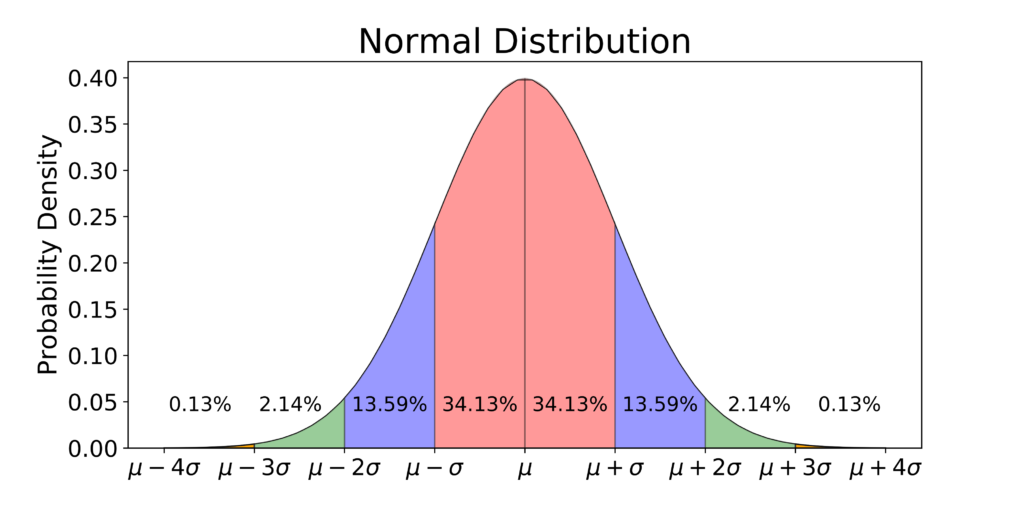
With the CDF defined as a function in python, we can now use it. We know that the total area under any PDF curve is 1 (this point will be discussed in more detail in a later section), which means the CDF across the whole range should be 1. Using 4 standard deviations away from each side of the mean adequately constitutes the whole range. Also, if we integrate starting from 4 standard deviations to the left all the way to the mean, we should calculate an area of 0.5. And, if we integrate from the mean all the way to 4 standard deviations to the right, we should also calculate 0.5. Let’s do these calculations for the 1^st graders’ heights, and for the IQ scores.

Code Block 3.7

text_1st = '1st Graders heights'
text_iqs = 'IQ scores'
values = [
    (text_iqs, 100, 15, 40, 160),
    (text_iqs, 100, 15, 40, 100),
    (text_iqs, 100, 15, 100, 160),
    (text_1st, 37, 2, 29, 45),
    (text_1st, 37, 2, 29, 37),
    (text_1st, 37, 2, 37, 45)]

for t in values:
    text = t[0]
    mean = t[1]
    std = t[2]
    lt = t[3]
    rt = t[4]
    cd_out = round(CDF(mean=mean, std_dev=std, 
                       x_left=lt, x_right=rt), 2)
    print(f'Probability of {text} being {lt} ≤ x ≤ {rt} is {cd_out}')

Above, we have used the CDF function repeatedly. The output from the above code block is shown in the below output block.

Probability of IQ scores being 40 ≤ x ≤ 160 is 1.0
Probability of IQ scores being 40 ≤ x ≤ 100 is 0.5
Probability of IQ scores being 100 ≤ x ≤ 160 is 0.5
Probability of 1st Graders heights being 29 ≤ x ≤ 45 is 1.0
Probability of 1st Graders heights being 29 ≤ x ≤ 37 is 0.5
Probability of 1st Graders heights being 37 ≤ x ≤ 45 is 0.5

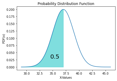
Now we can be confident that our “from scratch” PDF and CDF work, and that we understand the principles much more deeply. Let’s make sure we also know how to use the provided python modules such as norm.pfd(), and let’s also add some functionality that provides greater visualization (something that is always important for data scientists). The fill_between(X, y1, y2=0) method in matplotlib is used to fill the region between our left and right endpoints. Click here for a detailed overview of the function. (Here, y1 is the normal curve and y2=0 locates the X-axis). Here, we will find P(X ≤ 37) using the function norm.cdf(x, loc, scale).

Code Block 3.8

import scipy
import numpy as np
import matplotlib.pyplot as plt 
from scipy.stats import norm

X = np.arange(29, 46, 0.0001)
Y = norm.pdf(X, loc=37, scale=2)
plt.plot(X, Y)
plt.title("Probability Distribution Function")
plt.xlabel('X-Values')
plt.ylabel('PDF(x)')

# for fill_between
pX = np.arange(29, 37, 0.0001)  # X values for fill
pY = norm.pdf(pX,loc=37, scale=2)  # Y values for fill
plt.fill_between(pX, pY, alpha=0.5, color='c')  # Fill method call

# for text
prob = round(norm.cdf(x=37, loc=37, scale=2),2)
plt.text(34.5, 0.03, prob, fontsize=20)  # Add text at position
plt.show()

From the above code block, we get the following PDF with the integrated CDF value shown as the shaded area.

There are some important properties of Φ that should now be clear from all that was said above and should be kept in mind. For all x ∈ ℝ (the fancy way that we say for all x values that are real numbers), it is true that:

1. \Phi (0)=\frac{1}{2}
2. \Phi (-x)=1 - \Phi (x)
3. \lim\limits_{x \to +\infty} \Phi (x)=1
4. \lim\limits_{x \to -\infty} \Phi (x)=0

Let’s go over those individually remembering that the CDF is an integration from left to right of the PDF. Let’s start with properties 3 and 4. We shifted the mean to zero when we subtracted the mean of X from all values of X and we divided all those new values by the standard deviation. Therefore, when we integrate (we love that word on this blog) from -∞ to +∞, the result will be 1 (i.e. point 3 above). If we integrate from some very large negative number, the CDF will be 0 (i.e. point 4 above). If we only integrate up to 0 (property 1 above) instead of all the way to +∞, the result will be 1/2 (i.e. point 1 above). Consequently, looking at property 2 above, integrating up to any value of x must equal 1 – CDF of the opposite sign of that x.

Also, since Φ does not have a closed-form solution (meaning we can’t just calculate it directly, we must integrate programmatically to get the solution), it is sometimes useful to use upper and/or lower bounds. Since an infinite integral will not be considered as a closed-form, we need to define an upper and lower bound for the integration to get a definite CDF value. Refer to the solution of Problem 7 in this link to understand how the upper and lower bounds are defined. Please note that our above “from scratch code” does handle integrating from a specific left most value to a specific right most value.

4. Calculating Probabilities Using a Normal Distribution with Python Modules

Let’s now work through some examples of how we would find the probability of an event with respect to a constraint. For instance, we might want to estimate the probability of  < 700 mm of rain falling in the next 3 days. This can be written as P(x < 700), where x is a random variable from a data set X that shows the amount of rain in a particular area for a 3 month period each year. We can find this value by using the CDF. Let’s implement this in Python using the examples in the following sections.

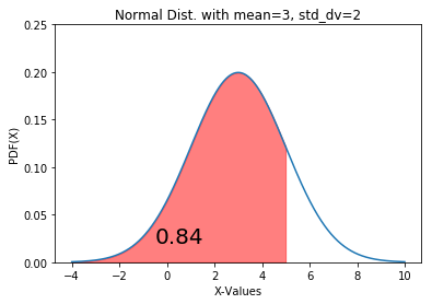
4.1 : To find P(X < x)

Given a population with mean 3 and standard deviation 2, we can find the probability P(X < 5) using the norm.cdf() function from SciPy. Here, in the function, the location (loc) keyword specifies the mean and the scale keyword specifies the standard deviation and x specifies the value we wish to integrate up to.

Continuing from the Calculating Probability using Normal Distributions in Python colab notebook above, the next block is

Code Block 4.1

from scipy.stats import norm

less_than_5=norm.cdf(x=5, loc=3, scale=2)
print(less_than_5)

The output from the above cell is

0.8413447460685429

The value 84.13% is the probability that the random variable is less than 5. In order to plot this on a normal curve, we follow a three-step process – plotting the distribution curve, filling the probability region in the curve, and labelling the probability value. We can achieve this using the following code:

Code Block 4.2

from matplotlib import pyplot as plt
import numpy as np
fig, ax = plt.subplots()

# for distribution curve
x= np.arange(-4, 10, 0.001)
ax.plot(x, norm.pdf(x, loc=3, scale=2))
ax.set_title("Normal Dist. with mean=3, std_dv=2")
ax.set_xlabel('X-Values')
ax.set_ylabel('PDF(X)')

# for fill_between
px=np.arange(-4,5, 0.01)
ax.set_ylim(0, 0.25)
ax.fill_between(px, norm.pdf(px, loc=3, scale=2), 
                alpha=0.5, color='r')

# for text
ax.text(-0.5, 0.02, round(less_than_5, 2), fontsize=20)
plt.show()

4.2 : To find P (x1 < X < x2)

To find the probability of an interval between two variables, you need to subtract one CDF calculation from another one when using norm.cdf. Let’s find 𝑃(0.2 < 𝑋 < 5) with a mean of 1, and a standard deviation of 2, (i.e. X ~ N (1, 2)).

Code Block 4.3

norm(1, 2).cdf(5) - norm(1,2).cdf(0.2)

This output for the above plot shows that there is a 63.2% probability that the random variable will lie between the values 0.2 and 5. To plot this, we can use the following code:

Code Block 4.4

fig, ax = plt.subplots()

# for distribution curve
x= np.arange(-6,8,0.001)
ax.plot(x, norm.pdf(x,loc=1,scale=2))
ax.set_title("Normal Dist. with mean=1, std_dv=2")
ax.set_xlabel('X-Values')
ax.set_ylabel('PDF(X)')
ax.grid(True)

px=np.arange(0.2,5,0.01)
ax.set_ylim(0,0.25)
ax.fill_between(px,norm.pdf(px,loc=1,scale=2),alpha=0.5, color='c')

pro=norm(1,2).cdf(5) - norm(1,2).cdf(0.2)
ax.text(0.2,0.02,round(pro,2), fontsize=20)
plt.show()

It’s worth noting that the code we wrote from scratch in python without numpy or scipy was able to perform a CDF integration between two values of a variable with one call. 

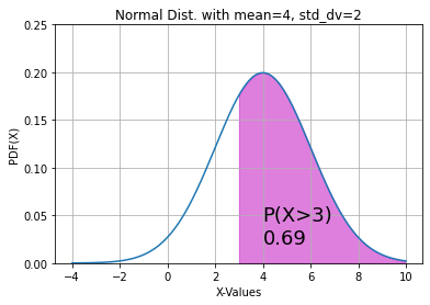
4.3 : To find P(X > x)

To find the probability of P (X > x), we can use norm.sf, which is called the survival function, and it returns the same value as 1 – norm.cdf. For example, consider that we have a population with mean = 4 and standard deviation = 2. We need to find P (X > 3). We can use the following code.

Code Block 4.5

greater_than_3 = norm.sf(x=3, loc=4, scale=2)
greater_than_3

The output of that block is 0.6914624612740131.

This probability can be plotted on a graph using the following code.

Code Block 4.6

fig, ax = plt.subplots()
x= np.arange(-4, 10, 0.001)
ax.plot(x, norm.pdf(x, loc=4, scale=2))
ax.set_title("Normal Dist. with mean=4, std_dv=2")
ax.set_xlabel('X-Values')
ax.set_ylabel('PDF(X)')
ax.grid(True)

px=np.arange(3, 10, 0.01)
ax.set_ylim(0, 0.25)
ax.fill_between(px, norm.pdf(px, loc=4, scale=2), 
                alpha=0.5, color='m')

ax.text(4, 0.02, "P(X>3)\n%.2f" %(greater_than_3), 
        fontsize=18)
plt.show()

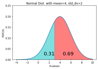
We explained the symmetric property of CDFs above. So, P(X > 3) can again be re-written as 1 – P(X < 3), i.e. P(X > 3) = 1 – P(X < 3). We can visualize this using the following code.

Code Block 4.7

gr4 = norm.cdf(x=3, loc=4, scale=2)
gr14 = 1-gr4
fig, ax = plt.subplots()
x= np.arange(-4, 10, 0.001)
ax.plot(x, norm.pdf(x, loc=4, scale=2))
ax.set_title("Normal Dist. with mean=4, std_dv=2")
ax.set_xlabel('X-values')
ax.set_ylabel('PDF(X)')


px=np.arange(3, 10, 0.01)
ax.set_ylim(0, 0.25)
ax.fill_between(px,norm.pdf(px, loc=4, scale=2), 
                alpha=0.5, color='r')
px1=np.arange(-4, 3, 0.01)
ax.fill_between(px1,norm.pdf(px1, loc=4, scale=2),
                alpha=0.5, color='c')
ax.text(4.5, 0.02, round(gr14, 2), fontsize=20)
ax.text(1, 0.02, round(gr4, 2), fontsize=20)
plt.show()

5. References

1. http://onlinestatbook.com/2/normal_distribution/history_normal.html
2. https://towardsdatascience.com/exploring-normal-distribution-with-jupyter-notebook-3645ec2d83f8

Closing

As we discussed above, while the normal distribution is common to measured data, it’s not the only type of distribution. There are tests that we can perform to measure the appropriateness of using the normal distribution. If the data fails the test for a normal distribution, there are other distributions that we can choose. We will cover these tests for normality and other distributions in upcoming posts.

Until next time …