Get the code and more on GitHub

Overview

If I had to describe Visual Python in one word, it would be “Elegance”. I first found it 20 years ago soon after I first started using Python. I was able to do amazing things with it right away, because it was and still is written that well.

Due to my overall background, I have a lot of experience in physics based modeling and controls system design. It was those realms that drove my rapid adoption and love of Visual Python (VP). I am finding that the unique qualities of Visual Python can now help me in my passion to better visualize data science work. Thus, I felt a post on VP would be good as a precursor to a tool that will be used at times in upcoming posts. I may even backtrack and use it to update some visualizations in previous posts.

The modeling for this post is not data science based as most people see data science. It is based in first principles physics using differential equations. It’s an interesting philosophical point that all first principles physics are based in usually simple and sometimes complex forms of basic data science techniques. If you do not have a background in modeling physical systems with differential equations, this post may seem hard. PLEASE do not let the modeling trip you up. Accept the physics equations (differential equations) for the physics as they are given and focus on the tool. That is the purpose of this post.

Why didn’t I may a first use to be data science based? I saw a post of an actual multi-pendulum system on LinkedIn from an AI influencer that I like to follow, and it occurred to me that modeling and animating that system using VP would be a great way for me to review and get back into VP, and to hopefully inspire others as to how VP can help them in their work.

The Physics

If you are not into physics based modeling, you can skip down to the equations at the end of this section to see the results. If you do have some background in physics due to your original field, I hope you find this to be a descent review. The free body diagram for pictorially describing the forces and constraints on one of our many pendulums is shown in figure 1 below.

A ball of mass m is acted upon by g and constrained to a circular motion by a chord that is r in length. According to Newton’s laws of motion, the mass will oppose changes in velocity with a force that is m r^2 \ddot{\theta} in magnitude. The ball will always have a force of m g on it. For any initial value of \theta, the ball will begin to move along the circular path that it is constrained to by the chord. At any moment in time, the ball will be constrained to the circular path by a force of m g r cos(\theta) (not shown in the diagram), and the ball will have a force of m g r sin(\theta) acting to move the ball to the state of \theta = 0, which is the equilibrium state (state of lowest overall system energy). There is one other force acting on the ball. It is proportional to the velocity of the ball as it moves through the air. The force causes energy to be lost from our pendulum system[s]. It would be \frac 1 2 \rho_{air} A_{cs ball} C_d (r {\dot \theta})^2. All terms except {\ddot{\theta}}^2 are constant and the product of those terms would be small. Thus, we will multiply {\omega}^2 by a small number to represent the energy lost from the pendulum as it moves back and forth along a semi-circular path through the air, which results in a decay of the peak positive and negative {\theta} state values. The sum of forces moving the ball along the path r \theta are

m g r sin(\theta) = m r^2 \ddot{\theta} + \frac 1 2 \rho_{air} A_{cs ball} C_d (r \dot{\theta})^2

Let’s make some simplifications and explanations before doing the algebraic preparation to prepare this equation for digital calculus we’ll need to simulate this small dynamic system. I believe that the term {\theta} is well understood to be the angle of the chord holding the ball m from vertical line. The term {\dot \theta} is the angular velocity and is sometimes called {\omega}. The term {\ddot \theta} is the angular acceleration and is sometimes called {\alpha}. In digital / numerical calculus, it’s convenient to use The term {\dot \theta} is the angular velocity and is sometimes called {\dot \omega} and {\ddot \omega} to note that we are using the first and second time derivatives of {\omega}, respectively. Let’s also (out of pure laziness and convenience) set the term \frac 1 2 \rho_{air} A_{cs ball} C_d (r {\dot \theta})^2 to f_d {\dot \theta}^2, where f_d = \frac 1 2 \rho_{air} A_{cs ball} C_d r^2 to make things easy. We should be fine as long as f_d is a reasonably small value. Our equation algebraically changed for numerical integration is

\ddot{\theta} = \frac g r sin(\theta) - f_d \dot{\theta}^2

We are at a good point now. Using the above equation, we can determine the acceleration of the ball at any state value \theta and \dot{\theta}. If we start the ball at some \theta, we we will assume that the initial state value for \dot{\theta} is zero, but you could have a non-zero value for \dot{\theta}. Let’s numerically integrate with very small time steps to determine \dot{\theta} and {\theta} at the next time step.

{\dot{\theta}}_i = {\ddot{\theta}}_{i-1} \delta t + {\dot{\theta}}_{i-1} {\theta}_i = {\dot{\theta}}_{i-1} \delta t + {\theta}_{i-1}

It’s worthy to note that I’ve used Newton’s method. There are other methods for finding a systems dynamic equations of motion such as Bond Graphs and Lagrangian methods.

Code without Visual Python

If we only wanted to solve the above differential equations for as many time steps as desired, we could use the code below.

import numpy as np
from Plot_Tools import Basic_Plot as BP

radius = 0.1
gravity = 9.81
f_d = 0.1

theta = np.pi / 3.0
theta_list = [theta]
theta_d = 0.0

time = 0.0
delta_t = 0.01
time_list = [0.0]
count = 0.0

while count < 10000:
    theta_dd = - gravity / radius * np.sin(theta) \
                - f_d * theta_d ** 2.0
    theta_d += theta_dd * delta_t
    theta += theta_d * delta_t

    theta_list.append(theta)
    time += delta_t
    time_list.append(time)

    count += 1

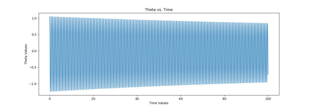
BP(x=time_list, y=theta_list,
   t='Theta vs. Time',
   x_t='Time Values', y_t='Theta Values')

The code above would yield the graph for Theta vs. Time below. Pendulums can swing for a long time. Especially ones that have a long chord. Trust me that the graph has a nice decaying sine wave. Better yet, run it for yourself. The BP class that was imported above is simply a plotting class developed in previous blog posts for convenience.

If we wanted to simulate multiple pendulums with progressively shorter (or longer) chords holding their respective masses, we could plot those too, but it would be kind of boring actually. What’s valuable is to watch a realistic dynamic animation of those pendulums. With a surprisingly small amount of additional code, we can do this. It is not hard to learn VP. It’s not even hard to master it, especially if you already know coding, or if you know Python well.

Code WITH Visual Python

Visual Python includes many examples with it’s install. You can install it with pip and anaconda. Their documents and tutorials and demos are pretty clear if you follow them in progressive order. If you’ve never seen VP code before, some of this may seem a little strange, but please just think of the VP parts as class instantiations and methods, because that is exactly what they are. This post is meant to be exactly what it is titled – an intro to VP. It is my hope that this post will help you determine if VP is a tool that you wish to add to your skill set.

Here are the major pieces of the VP code for animating multiple pendulums.

1. Imports for Visual Python and Numpy
2. A function to create a rainbow of colors for the pendulum balls, so that each pendulum ball has a unique color
3. Parameters for the visual python objects
4. Parameters to control the gradual changes in pendulums
5. Initiation of storage arrays to hold information for the pendulums
6. Length parameter for the mount that the pendulums will connect to and a call to the VP box class to instantiate the mount object
7. A call to the get_color_vectors function described above
8. A for loop that
   a) calculates the radii for each pendulum chord,
   b) makes calls to the VP cylinder class to draw a chord for each pendulum with each color
   c) makes calls to the VP sphere’s class to draw each ball with each color
9. The Dynamic Section:
   a) Parameters for the physics
   b) Parameters for the numerical simulation
   c) Initialization of the state variables
   d) A while loop to control the time steps of the numerical simulation
   e) A for loop to update rotation about the mounts for each pendulum,
   and to update the state variables using numerical integration.

The code below has the same comments in it as the above list. While the above list is hopefully clear from a high level, there is one non-standard thing in the code below to watch for. The rotation of Visual objects happens using the incremental changes in {\theta}. They do not use \dot{\theta} directly. This is something to watch out for when you are simulating state variables for physical systems.

from vpython import *
import numpy as np
import sys
import time


# Function to create a rainbow of colors for the pendulum balls
def get_color_vectors(num_of_pendulumns):
    color_step_size = 2.0 / num_of_pendulumns

    def val_adjust(val):
        if val < 0.0:
            val = 0.0
        elif val > 1.0:
            val = 0.0

        return val

    color_vectors = []
    rnd_amt = 3

    for i in range(num_of_pendulumns):
        vals = 1.0 - color_step_size * i

        val1 = val_adjust(round(+vals, rnd_amt))

        val2a = val_adjust(round(1.0 + vals, rnd_amt))
        val2b = val_adjust(round(1.0 - vals, rnd_amt))
        val2 = val2a + val2b
        val2 = 1.0 if val2 > 1.0 else val2

        val3 = val_adjust(round(-vals, rnd_amt))

        color_vectors.append(vector(val1, val2, val3))

    return color_vectors


# Parameters for the visual python objects
ball_radius = 0.4
num_of_pendulumns = 20
pend_step_size = 0.5
chord_var = 2.0  # overall chord variation - shortest to longest
middle_chord = 10.0

# Parameters to control the gradual changes in pendulums
pend_step = num_of_pendulumns * pend_step_size / (num_of_pendulumns - 1)
radius_step = chord_var / (num_of_pendulumns - 1)

# Initiation of storage arrays to hold information for the pendulums
colors = []
radii = []
chords = []
balls = []

# Length parameter for the mount that the pendulums will connect to and a
#     call to the VP box class to instantiate the mount object
length = num_of_pendulumns * pend_step_size + 1.0
mount_ht = middle_chord / 2.0 + ball_radius / 2.0
mount = box(pos=vector(0, mount_ht, length / 2.0),
            axis=vector(0, 0, length),
            width=ball_radius,
            height=ball_radius)

# The call to the get_color_vectors function
color_vectors = get_color_vectors(num_of_pendulumns)

# For each pendulum, calc the radius, and draw its chord and ball
for i in range(num_of_pendulumns):
    radii.append(middle_chord - chord_var / 2.0 + i * radius_step)

    chords.append(cylinder(pos=vector(0, middle_chord / 2.0,
                                      pend_step * i + pend_step_size),
                           axis=vector(0, -radii[-1], 0),
                           radius=0.025,
                           color=color.white))

    balls.append(sphere(radius=0.4,
                        pos=vector(
                            0,
                            middle_chord / 2.0 - radii[-1],
                            pend_step * i + pend_step_size),
                        color=color_vectors[i]))

time.sleep(4)
###############################################################################
# Dynamic Section
# Parameters for the physics
gravity = 9.81
f_d = 0.01

# Parameters for the numerical simulation
count = 0.0
delta_t = 0.01

# Initialization of the state variables
theta = [np.pi / 3.0] * num_of_pendulumns
theta_steps = [np.pi / 3.0] * num_of_pendulumns
theta_d = [0.0] * num_of_pendulumns
theta_dd = [0.0] * num_of_pendulumns

# A while loop to control the time steps of the numerical simulation
while count < 1000000:
    rate(150)

    # Update rotation about the mounts for each pendulum
    for i in range(num_of_pendulumns):
        chords[i].rotate(angle=theta_steps[i],
                         axis=vector(0, 0, 1))

        balls[i].rotate(angle=theta_steps[i],
                        axis=vector(0, 0, 1),
                        origin=vector(
                            0,
                            + middle_chord / 2.0,
                            pend_step * i + pend_step_size))

        # Update the state variables using numerical integration
        theta_dd[i] = - gravity / radii[i] * np.sin(theta[i]) \
            - f_d * theta_d[i] ** 2
        theta_d[i] += theta_dd[i] * delta_t
        theta_steps[i] = theta_d[i] * delta_t  # for VP object movements
        theta[i] += theta_steps[i]

    if count == 0:
        sleep(4)

    count += 1

Watching the Animation

Now for the good part – watching the animation. I’ve provided a video below, but it would really be best if you clone the repo and run it yourself after installing Visual Python.

Closing

In many future posts, and possibly some past posts, Visual Python will be incorporated to provide helpful visualizations of our work. This is a very powerful tool. Even the tools and visualizations that I was able to create with VP 20 years ago would seem impressive today, and I assure you it was less to do with my talent and more to do with this great module. I hope it can help you in your work too. Until next time …