Find the Files on GitHub

Overview

You may have been expecting Lasso, or Ridge, or Elastinet, or PCA, or some metrics for models so that we could compare models, etc. Why a clustering post? I sympathize completely. In short, it’s all part of a larger plan, and posts for those other topics are in the works or on the blog post road map. But, even IF you were hoping for a different flavored post, I believe that you will find this post to be more fun than data scientists should be allowed to have.

REMINDER

This blog is not about some vain attempt to replace the AWESOME sklearn classes. It is about understanding, among other things, how one might go about coding such tools without using scipy or numpy, so that we can someday gain greater insights, AND have a clue what to do, IF we need to advance or change the tools somehow.

With regard to our standard reminder above, it is my goal to make our classes much like the sklearn classes. For simplicity (and maybe laziness), I did not do that as much this time. However, one could easily take what we’ll present to a state more like the cluster class from sklearn.

The Points / Math / Code … Uuuh!

What I mean is, we usually go over math, then code, then output and compare to sklearn module output. With clustering, it just makes sense to start with a scatter plot and then just talk about the math and the code and the intermediate scatter plots all at the same time. So we’ll just jump into it all the pieces in an integrated fashion.

Our Initial Points

The scatter plot below shows the fake data that we will start with, and that we will use to illustrate the progress of the clustering class that we will develop together.

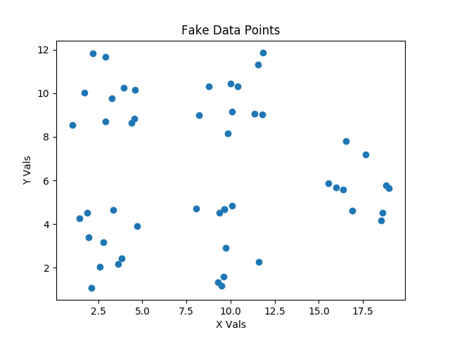
In the KMeans.py file in the GitHub Repo there is a CreateFakeData class. As always, I hope that you have already cloned or downloaded a copy of this repo. Please take a look at the CreateFakeData class on your own. It’s really pretty simple, and it makes our validation work for various types of fake clustering very easy.

NOTE

The code presented herein has almost no comments. This is for economy of space and the post is describing the code anyway. The code on the repo will have much more commentary and documentation inside the code.

An Overview of Our Code

The image below is a screen shot of my sublime text editor window that shows the high level class structure. I would have put this in a code window, but I was too lazy to do all the editing to make that work right. I hope this is palatable to you guys.

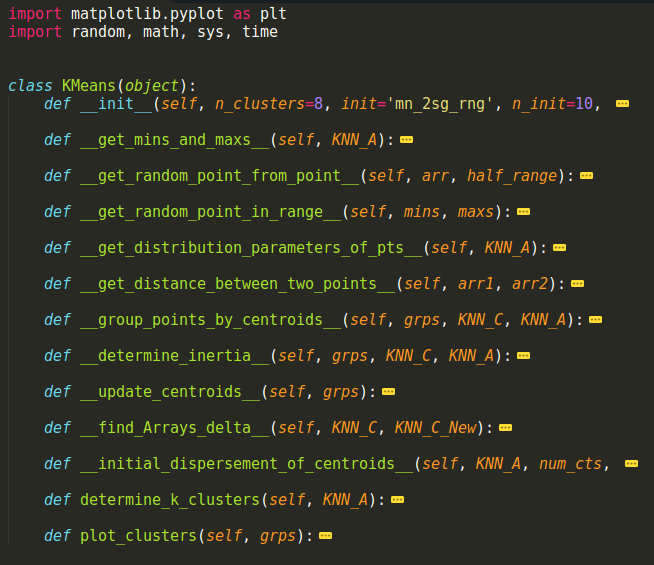
We’ll go through each of these functions below, but I will start with the determine_k_clusters method first. We’ll then cover each of the other methods in the order that they get called.

determine_k_clusters

    def determine_k_clusters(self, KNN_A):
        min_inertia = 1e10
        for attempt in range(self.n_init):
            KNN_C = self.__initial_dispersement_of_centroids__(
                KNN_A, self.n_clusters)
            
            # Loop beginning
            cnt = 0
            while cnt < self.max_iter:
                grps = {}
                for i in range(self.n_clusters):
                    grps[i] = {'centroids':[], 'points':[]}

                # Find groups by closest to centroid
                grps = self.__group_points_by_centroids__(grps, KNN_C, KNN_A)
                
                KNN_C_New, grps = self.__update_centroids__(grps)

                delta_As = self.__find_Arrays_delta__(KNN_C, KNN_C_New)
            
                if delta_As == 0:
                    break

                KNN_C = KNN_C_New
                
                cnt += 1

            #######
            current_inertia = self.__determine_inertia__(grps, KNN_C, KNN_A)
            if current_inertia < min_inertia:
                min_inertia = current_inertia
                grps_best = grps

        self.inertia_ = min_inertia

        return grps_best

Luckily, the above method is one of the longer ones, and it’s not bad. I usually divide the code into sections to discuss, but that would litter this code with too many comments. Each line needs to be discussed, and the extra white space is there for clarity.

1. I’ll first describe the steps with writing and bold word Numbers, such as First, Second, etc., and
2. then we’ll go back over the steps using descriptive images that better illustrate them, and
3. then will review the details of each of the private methods in sub-sections, which will have titles that start with the bold word Numbers.

First, we pass our list of cluster points, which are constantly preserved in the KNN_A array of points, into this method, and those points can be of any dimension.

Second, we initialize the min_inertia variable with a ridiculously high value, so that it will be set to the first calculated inertia from our first clustering pass.

Third, we start the attempt for loop, which will run n_init times. Why? Automatic clustering methods rely on an initial set of randomly generated centroid locations that will MOST certainly NOT be the final centroid locations. Sometimes those initial positions will not migrate to the optimal cluster centers due to their poor initial placement. In such cases, the inertia results for the entire set of clusters (calculation to be discussed below) will be higher than in those cases where the centroids do migrate to the optimal locations. We keep track of which centroid and cluster groups resulted in the minimum inertia, and we use those centroids and cluster groups as our answer.

Fourth, the first task inside the for loop is to determine an __initial_disbursement_of_centroids__. There are different ways to randomly initialize these centroid locations, but all of them can result in missing the optimal clustering as previously described.

Fifth, with our initial centroids in hand, we enter a while loop that will continue no more than max_iter times until the centroids stop moving between steps. An empty grps dictionary is initialized to organize our centroids and their associated points.

Sixth, we then place our points stored in KNN_A into groups associated with the centroids according to, which centroid they are closest to, and we do this with the __group_points_by_centroids__ method.

Seventh, now that the points have been divided into clusters, we can determine the centers of those clusters with __update_centroids__ , which returns both the updated grps dictionary and a KNN_C_new array of centroids.

Eighth, we send KNN_C and KNN_C_new into __find_Arrays_delta__ to check their overall distances from each other.

While Loop Final Statements either: A) break out of the while loop if the KNN_C and KNN_C_new arrays are equal; or B) update KNN_C to KNN_C_new if they are NOT equal, advance the count of the while loop, and continue the while loop to find optimal centroid locations.

For Loop Final Statements check to see if the current inertia of all the centroids is the minimum inertia (the actual minimum is HIGHLY likely to reoccur many times). If the current inertia is the minimum inertia so far, the min_inertia variable is updated, and the grps_best dictionary is updated, which associates the centroid locations of each cluster to their respective cluster points.

The Final Method Statements simply assign the minimum inertia to the self.min_inertia_ attribute for our class and return the best grouping of centroids stored in grps_best.

Scatter Plot Version of determine_k_clusters

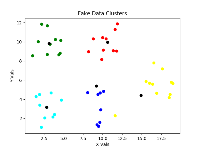
First we start with data we hope to organize into clusters as in figure First.

For the Second thru Sixth steps, we’ve 2) initialized our min_inertia variable, 3) entered our attempt for loop, 4) created an initial random dispersion of our centroids shown in black, 5) entered our centroid optimization while loop, and 6) grouped points by nearness to the initial centroids with different colors to illustrate the current clusters. What a clump of steps! It just seemed like the best “next GROUP of steps” for an image update.

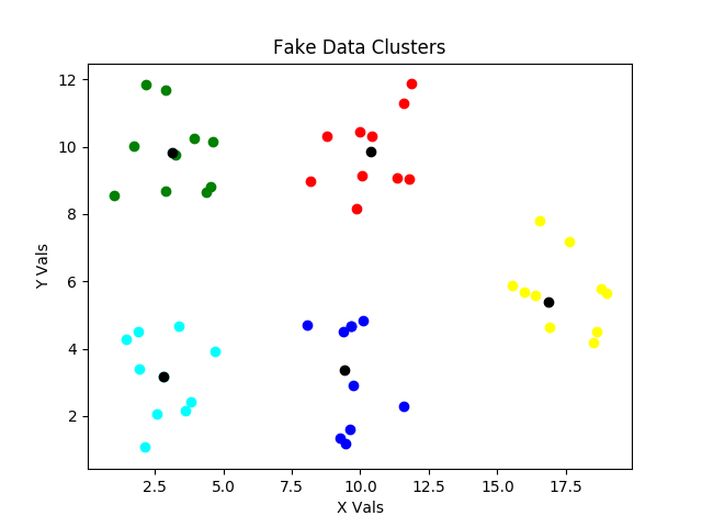
For the Seventh step and back around to Sixth step, we’ve updated the centroid locations to be in the center of the initial clustering, and then reassessed, which points are closest to which centroids. Notice the slight reassignments of centroid locations and of points to clusters in the latest two scatter plots above.

Continuing through the for loop causes an adjustment of centroid locations, and and adjustment of, which points belong to the clusters defined by those centroids.

In the version C figure above, there are only small changes in assignments of points to clusters, but there are still significant changes of centroid locations.

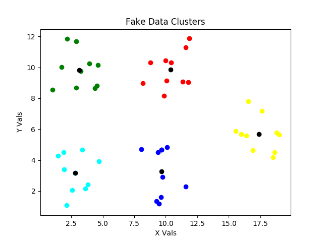
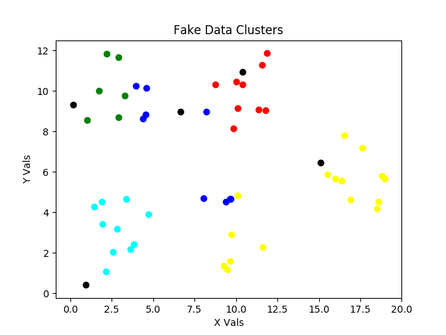
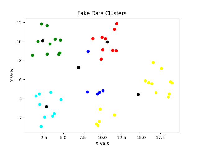
The final small change between the versions C and D figures is the location of the centroid for the cluster denoted by yellow, and our clusters are then optimized and the inertia is minimized. But this is just the end of our first while loop optimization. We start this process COMPLETELY over in the next attempt for loop iteration. Why? Those clusters look AWESOME! Well, as explained above, they don’t always look awesome. The initial randomized locations for centroid locations can result in poor clustering, and we don’t want to have to baby sit the routine, so we perform multiple attempts and choose the clustering with the minimum inertia as also described above. What do poor clusterings look like?

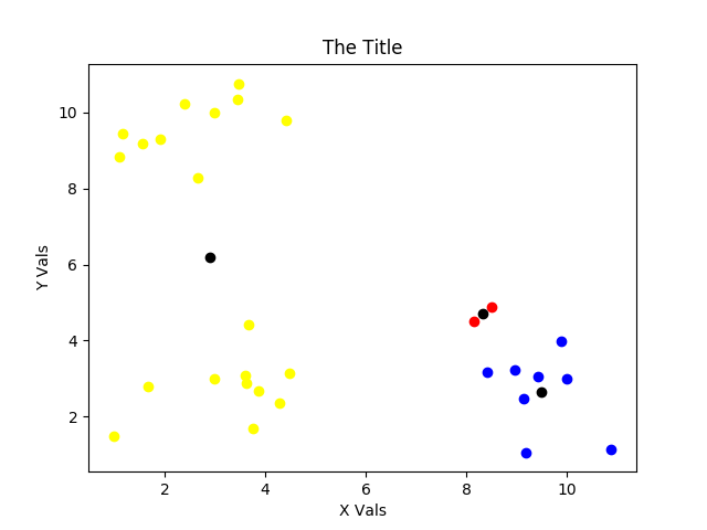
Oh my! Yeah. The math and optimization are correct for the choice of initial centroids, but this clustering is poor. It’s a kin to local vs. global minima and using a “Monte Carlo” method to help us get out of it. Hence, the attempt for loop is there to serve as our pseudo Monte Carlo method to make sure we do NOT get something like what is shown in the above figure. If we didn’t have a way to calculate and compare inertias, we’d have to baby sit this process in order to avoid such situations.

Furthermore, our fake data was arranged into clearly defined clusters. We still have to run our clustering routine for a variable number of clusters and observe each clustering to humanly determine, which amount of clusters makes the most sense. Sometimes the clustering is obvious. Sometimes you just have to do the best that you can to “draw the lines” (i.e. determine which number of clusters is best for your situation).

Fourth __initial_disbursement_of_centroids__

MOST of the code for the __initial_disbursement_of_centroids__ private method is shown below. There is an elif block below this code in the same private method, and you can see that once you download or clone the code from the repo. Why not show it all? We could, just like sklearn, have multiple methods for initially assigning centroid locations. The one that I am showing works fine. The second method that I am not showing works as well or better SOME OF THE TIME, but not always. In short, there’s an art to such things, and no one method is better than all the rest … yet! If I find one that never results in the trap shown above, I will share it. For now, all methods are simply different ways to randomly initialize centroid locations, and I felt that it was best to just cover one (or I was lazy and didn’t want to show more than one … I think it’s a little of both).

    def __initial_disbursement_of_centroids__(self, KNN_A, num_cts, 
        method='mn_2sg_rng'):
        means, stds = self.__get_distribution_parameters_of_pts__(
            KNN_A)
        
        two_sig  = []
        for element in stds:
            two_sig.append(element*2.0)

        KNN_C = []

        if method == 'mn_2sg_rng':
            for i in range(num_cts):
                KNN_C.append(
                    self.__get_random_point_from_point__(
                        means,two_sig))

            return KNN_C

A quick review of the above method will show you that this private method relies on two other private methods, which are each pretty simple. We’ll cover them after discussing this method at a high level.

1. Notice that we send in the points to be clustered as KNN_A, the number of centroids as num_cts, and the method name as method=’string of method name’.
2. Next, we use the __get_distribution_parameters_of_pts__ to get the means and standard deviations for all the dimensions of all the points.
3. We create a two_sig array (i.e. an array of two standard deviations for each dimension) to help with our creation of random centroids.
4. Finally, we pass the means and two_sig arrays into the __get_random_point_from_point__ private method repeatedly in the for loop inside the if block to get num_cts random centroids.

The __get_distribution_parameters_of_pts__ private method is shown below.

    def __get_distribution_parameters_of_pts__(self, KNN_A):
        num_pts = len(KNN_A)
        number_of_dimensions = len(KNN_A[0]) 

        means = [0] * number_of_dimensions
        stds  = [0] * number_of_dimensions

        # Determine means for each dimension
        for arr in KNN_A:
            for i in range(number_of_dimensions):
                means[i] += arr[i]
        for i in range(number_of_dimensions): 
            means[i] /= num_pts

        # Determine standard deviations for each dimension
        for arr in KNN_A:
            for i in range(number_of_dimensions):
                stds[i] += (means[i] - arr[i])**2
        for i in range(number_of_dimensions): 
            stds[i] = (stds[i] / num_pts)**0.5

        return means, stds

I trust the operations of the above method are clear. We are simply:

1. Receiving all the points that are being used in the clustering exercise.
2. Initializing two parameters for use in the for loops.
3. Initializing two arrays to hold our statistics for each dimension.
4. Performing two for loop operations to determine our means.
5. Performing two for loop operations to determine our standard deviations.
6. Returning our statistics.

The handy __get_random_point_from_point__ private method is below.

    def __get_random_point_from_point__(self, arr, half_range):
        number_of_dimensions = len(arr)

        pt = []
        for i in range(number_of_dimensions):
            var = random.uniform(-half_range[i],half_range[i])
            pt.append(arr[i]+var)

        return pt

It does the following steps:

1. Receives an array of points as arr, and an array of half ranges as half_range.
2. Establishes a parameter for our one for loop, which is the number of dimensions as number_of_dimensions.
3. Establishes an empty array named pt, which we will later return.
4. For each dimension, it first gets a random variable var between a negative and positive value of the current half_range, adds this to the current array value of arr, which is a mean for each dimension, and appends the result to pt for eventual return once complete.

This completes our coverage of how we initialize our centroid locations. Phew!

Sixth group_points_by_centroids

Now we simply figure out, which centroid each point is closest to, and we define the clusters accordingly. The __group_points_by_centroids__ is shown below.

    def __group_points_by_centroids__(self, grps, KNN_C, KNN_A):
        for pta in KNN_A:
            minD = 1e10
            for i in range(len(KNN_C)):
                ptc = KNN_C[i]
                dist = self.__get_distance_between_two_points__(
                    ptc, pta)
                if dist < minD:
                    closest_centroid = i
                    minD = dist

            grps[closest_centroid]['points'].append(pta)
            if grps[closest_centroid]['centroids'] == []:
                grps[closest_centroid]['centroids'] = \
                    KNN_C[closest_centroid]

        return grps

Let’s step through the above private method.

1. We’ve passed in the grps dictionary, which has centroid and points for each current cluster, the array of centroid locations (KNN_C), and the array of points (KNN_A). It’s convenient to have the KNN_A and KNN_C arrays separate, even though they are inside grps, for updating reasons. This way the centroids and points can be regarded independently from the cluster groups in grps.
2. The first for loop steps through each of our points, and we set minD, which stands for minimum distance, to be ridiculously large, so that it will be reset in the first iteration, and according to comparison logic afterwards.
3. The nested, second, for loop is used to determine the distance, dist, of the current point to each centroid using the private method __get_distance_between_two_points__. The if block helps us track, which centroid is closest to the current point.
4. Once the nested, second, for loop is complete, the grps dictionary is updated with the cluster that point belongs to, and a centroid location for that cluster is also added.
5. Once all points have been grouped with the centroid that they are closest to, the grps dictionary is returned.

The __get_distance_between_two_points__ private method is shown below.

    def __get_distance_between_two_points__(self, arr1, arr2):
        sq_dist = 0
        for i in range(len(arr1)):
            sq_dist += (arr1[i] - arr2[i])**2

        return sq_dist**0.5

1. Two points of any dimension are passed in.
2. We sum the squares of the difference for each dimension between the two points.
3. Finally, we return the square root of the summed differences.

Seventh __update_centroids__

With the points updated into clusters in accordance with the centroids they are closest to, we can move the centroids to the centers of those clusters. The private method __update_centroids__ does this and is shown below.

    def __update_centroids__(self, grps, KNN_A):
        KNN_C_New = []
        total_number_of_clusters = len(grps)
        number_of_dimensions = len(KNN_A[0])
        mins, maxs = self.__get_mins_and_maxs__(KNN_A)
                
        for i in range(total_number_of_clusters):
            number_of_points_in_cluster = len(grps[i]['points'])
            if number_of_points_in_cluster == 0: 
                # assign that centroid a new random location
                KNN_C_New.append(
                    self.__get_random_point_in_range__(mins,maxs))
                grps[i]['centroids'] = KNN_C_New[-1]
                continue # then continue
                
            cnt_locs = [0] * number_of_dimensions

            for j in range(number_of_dimensions):
                for k in range(number_of_points_in_cluster):
                    cnt_locs[j] += grps[i]['points'][k][j]
                cnt_locs[j] /= number_of_points_in_cluster

            grps[i]['centroids'] = cnt_locs
            KNN_C_New.append(cnt_locs)

        return KNN_C_New, grps

In a perfect analytical world, this method could have been much shorter, but there was a need to deal with those pesky times that an initial centroid ends up with no points associated with it. The statements inside the if block that is inside the outer for loop “kicks” a centroid, that has no points associated with it, to a new location. This usually does the trick and allows the centroid to pick up some points on the next iteration. Let’s step through this method.

1. The current grps dictionary is passed in.
2. An empty KNN_C_new array is initialized for storage.
3. We establish a total_number_of_clusters parameter for convenience.
4. Determine the number of dimensions for the points to be used later.
5. Also for convenience, minimums and maximums for each dimension from all points (mins, maxs) are found and stored.
6. We run the outer for loop total_number_of_clusters times.
7. We set a number_of_points_in_cluster parameter for each iteration of this outer for loop.
8. IF there are no points in the current cluster (well darn) use __get_random_point_in_range__ with mins and maxs as a range to find a new random location for the centroid in hopes that the new centroid will recruit some points into its cluster in the next iteration. Add this new point to the KNN_C_new array and to the grps dictionary, and continue to the next step of the outer for loop.
9. Initialize an array named cnt_locs (short for centroid locations) that is all 0’s and that will store our NEW centroid locations that will be located in the center of the current cluster groupings.
10. Enter the next group of for loops that cycle through each dimension of each point in the current cluster. These two for loops work together to find the average location, effectively the point at the center, of the current cluster, and assign that point to be the updated centroid of the cluster. This new point is appended to KNN_C_new, and the grps dictionary is updated with it for that cluster, and these are returned.

The __get_mins_and_maxs__ private method is shown below.

    def __get_mins_and_maxs__(self, KNN_A):
        number_of_points = len(KNN_A)
        number_of_dimensions = len(KNN_A[0])

        mins = [1e10] * number_of_dimensions
        maxs = [-1e10] * number_of_dimensions

        for i in range(number_of_points):
            for j in range(number_of_dimensions):
                if KNN_A[i][j] < mins[j]:
                    mins[j] = KNN_A[i][j]
                if KNN_A[i][j] > maxs[j]:
                    maxs[j] = KNN_A[i][j]

        return mins, maxs

This is pretty basic, but let’s go over it for clarity:

1. Establish two useful parameters, number_of_points and number_of_dimensions, for our for loops and to help in initializing our storage arrays for mins and maxs for each dimension.
2. Initialize our mins and maxs arrays with values that will surely get reset on first consideration.
3. For each point, and for each dimension of each point, see if we can update the minimum or maximum value for that dimension.
4. Return the mins and maxs when done.

These mins and maxs are then passed into __get_random_point_in_range__ for those times that we need to “kick” a centroid with no points associated to it (a lonely centroid is a sad centroid) to a new random location. Again, this is in hopes that it will pick up some points on the next iteration. Let’s look at the __get_random_point_in_range__ private method.

    def __get_random_point_in_range__(self, mins, maxs):
        pt = []
        for i in range(len(mins)):
            pt.append(random.uniform(mins[i],maxs[i]))

        return pt

In summary, this method is finding a random number from the min and max for each dimension and appending it to our pt array that was initialized as an empty array.

Eighth __find_Arrays_delta__

With KNN_C_new in hand from above, we can compare it to KNN_C using __find_Arrays_delta__. This private method is shown below.

    def __find_Arrays_delta__(self, KNN_C, KNN_C_New):
        dist_sum = 0
        for i in range(len(KNN_C)):
            dist_sum += self.__get_distance_between_two_points__(
                KNN_C[i], KNN_C_New[i])

        return dist_sum

This routine is finding the distance between the last centroid locations and the updated centroid locations by using the method called __get_distance_between_two_points__ that we covered previously. It’s doing this for each centroid, old and new, and then summing the differences.

Final Steps

Even though we covered the final steps of determine_k_clusters above, let’s review them briefly here.

1. If the KNN_C‘s are the same as the KNN_C_new‘s, we break out of the while loop before the max_iter count is reached.
2. If we’ve completed all n_init attempts, we choose the solution with the minimal inertia.

Let’s look at the technique to calculate that inertia found in the private method __determine_inertia__.

    def __determine_inertia__(self, grps):
        inertia = 0
        for i in range(len(grps)):
            for j in range(len(grps[i]['points'])):
                dist = self.__get_distance_between_two_points__(
                        grps[i]['centroids'], 
                        grps[i]['points'][j])
                inertia += (dist) ** 2

        return inertia

The steps for this method are:

1. Initialize the inertia variable to 0 that will be returned at the end of the process.
2. For each cluster …
3. For each point in a cluster …
4. Find the distance between the centroid for that cluster and the current point.
5. Square this distance for each difference and add it to the running total.
6. The final total is returned as the inertia.

Other Files and Methods and Functions

There is one final method that plots the clusters. Surprisingly, it is named plot_clusters. It only works for two dimensions. There is a similar function outside the class structures called scatter_plot_points to be used to scatter plot points in general. If you run KMeans.py, it will run everything and present an initial plot. Once you close this, it will continue to run and present a final plot. The Kmeans_Initial.py file was the initial development file for this work. I share it in case it can be helpful. The skl_kmeans_compare.py file was used to compare sklearn clustering on similar data to our pure python version, and they do compare well. Finally, the Mall_Customers.csv file is some practice data that can be applied to clustering routines for further practice.

Closing

My plan is to bring this blog and the previous blogs into an interesting bit of hybrid work. I may hit some walls with those efforts. If so, I will postpone reports on that work until it gets to a practical point for sharing. I am also hoping to find a new breakthrough with certain aspects of k means. In a perfect world, that would be my next post. Hopefully, things will go close enough to perfect, that I can confirm that breakthrough and communicate it soon. Regardless, I feel like I am having more fun than I should be allowed to have.

Until next time …