Find the files on GitHub

Overview

In this post, we have an “integration” of the two previous posts. Now, we make sure that the polynomial features that we create with our latest polynomial features in pure python tool can be used by our least squares tool in our machine learning module in pure python. Here’s the previous post / github roadmap for those modules:

Blog Posts	GitHub Repo’s
Pure Python Machine Learning Module: Polynomial Tools Class	LeastSquaresPolyFit PurePy
Pure Python Machine Learning Module: Least Squares Class	MachineLearningModule PurePy

REMINDER

This blog is not about some vain attempt to replace the AWESOME sklearn classes. It is about understanding, among other things, how one might go about coding such tools without using scipy or numpy, so that we can someday gain greater insights, AND have a clue what to do, IF we need to advance or change the tools somehow.

The Test Code

This post feels a bit strange, because we so often go over some math theory and then show how to apply that math theory using python code. This time, we will only be reviewing test code that uses those two previously developed tools. Please go to the GitHub repo for this post and “git” the code so you can follow along in your favorite editor. For those otherwise positioned at the moment, I will still show all the code below.

Test Code 1

I’ve broken the test files down into sections noted by comments. The first file is named LeastSquaresPolyPractice_1.py in the repository. Section 1 prepares the fake data for usage. Note that it is not in the correct format just yet, but we will get it there soon. We’re also begin preparing a plot for the final section. In Section 2, the fake data is put into the proper format. In Sections 3 and 4, the fake data is prepared to be put into our desired polynomial format and then fit using our least squares regression tools using our pure python and scikit learn tools, respectively. Section 5 compares the coefficients, and while they are in a different order, each method gets the same coefficients. Then, in Sections 6, we compare the two methods again, but on new fake data using the original fits for each method. Section 7 compares the outputs and Section 8 shows the final graph. These last two sections are discussed in more detail below.

import LinearAlgebraPurePython as la 
import MachineLearningPurePy as ml

from sklearn.linear_model import LinearRegression
from sklearn.preprocessing import PolynomialFeatures

import matplotlib.pyplot as plt


# Section 1: Fake data preparation 
#   and visualization
X = [2,3,4]
def y_of_x(x):
    return 0.2*x + 0.5*x**2
Y = []
for x in X:
    Y.append(y_of_x(x))

print('Calculated Y Values:', Y, '\n')

plt.scatter(X, Y)

# Section 2: Get fake data in correct format
X = la.transpose([X])
Y = la.transpose([Y])

# Section 3: Pure Python Tools Fit
poly_pp = ml.Poly_Features_Pure_Py(order=2)
Xpp = poly_pp.fit_transform(X)
ls_pp = ml.Least_Squares(add_ones_column=False)
ls_pp.fit(Xpp, Y)

# Section 4: SciKit Learn Fit
poly_sk = PolynomialFeatures(degree = 2)
Xsk = poly_sk.fit_transform(X)
ls_sk = LinearRegression()
ls_sk.fit(Xsk, Y)

# Section 5: Coefficients Comparison
formatted_lsp_coefs = [round(x,9) 
    for x in la.transpose(ls_pp.coefs)[0]]
print('PurePy  LS coefficients:', formatted_lsp_coefs)
print('SKLearn LS coefficients:', ls_sk.coef_, '\n')

# Section 6: Create Fake Test Data
XLS = [0,1,2,3,4,5]

# Section 6.1: Predict with Fake Test Data
#   Using Pure Python Tools
XLS_pp = poly_pp.transform(la.transpose([XLS]))
YLS_pp = ls_pp.predict(XLS_pp)
YLS_pp = la.transpose(YLS_pp)[0]

# Section 6.2: Predict with Fake Test Data
#   Using SciKit Learn Tools
new_X = poly_sk.transform(la.transpose([XLS]))
YLS_sk = ls_sk.predict(new_X)
YLS_sk = YLS_sk.tolist()
YLS_sk = la.transpose(YLS_sk)[0]

# Section 7: Calculate Prediction Differences 
deltas = [ YLS_pp[i] - YLS_sk[i] 
    for i in range(len(YLS_pp)) ]
print( 'Prediction Deltas:', deltas , '\n')

# Section 8: Plot Both Methods
plt.plot(XLS, YLS_pp, XLS, YLS_sk)
plt.xlabel('X Values')
plt.ylabel('Y Values')
plt.title('Pure Python Least Squares Line Fit')
plt.show()

Below is the output from the above code including the output graph. Note that the two methods, pure python and scikit learn, are so close, that the prediction deltas are extremely small, and the two graph lines through the initial fake data points are one on top of the other.

Calculated Y Values: [2.4, 5.1, 8.8] 

PurePy  LS coefficients: [0.5, 0.2, 0.0]
SKLearn LS coefficients: [[0.  0.2 0.5]] 

Prediction Deltas: [2.1516122217235928e-13, 
8.670841822322473e-14, 8.881784197001252e-15, -1.7763568394002505e-14, 7.105427357601002e-15, 8.348877145181177e-14] 

Test Code 2

This next file we’ll go over is named LeastSquaresPolyPractice_2b.py in the repository. It is laid out the same as the previous file. The 2a version is a bit simpler in that the fake data does not have random noise added into the output. We’ll discuss how the outputs differ below. Section 1 prepares the fake data and plotting; Section 2 formats the input and output data; Sections 3 and 4 put the fake data into our desired polynomial format and fits a solution using our pure python and scikit learn tools, respectively; Section 5 compares the coefficients; Sections 6 compares the two tool sets on fake test data using the original fits; Section 7 compares outputs; and Section 8 shows the final graph. As before, these last two sections are discussed below the code.

import LinearAlgebraPurePython as la 
import MachineLearningPurePy as ml

from sklearn.linear_model import LinearRegression
from sklearn.preprocessing import PolynomialFeatures

import matplotlib.pyplot as plt
import random


# Section 1: Fake data preparation 
#   and visualization
X = [float(x)/20.0 for x in range(100)]
def y_of_x(x):
    return 0.2*x + 0.7*x**2 + random.uniform(-1,1)
Y = []
for x in X:
    Y.append(y_of_x(x))

plt.scatter(X, Y) # sys.exit()

# Section 2: Get fake data in correct format
X = la.transpose([X])
Y = la.transpose([Y])

# Section 3: Pure Python Tools Fit
poly_pp = ml.Poly_Features_Pure_Py(order=2)
Xpp = poly_pp.fit_transform(X)
ls_pp = ml.Least_Squares(tol=2, add_ones_column=False)
ls_pp.fit(Xpp, Y)

# Section 4: SciKit Learn Fit
poly_sk = PolynomialFeatures(degree = 2)
Xsk = poly_sk.fit_transform(X)
ls_sk = LinearRegression()
ls_sk.fit(Xsk, Y)

# Section 5: Coefficients Comparison
tmp_ls_pp_coefs = sorted(ls_pp.coefs)
rounded_ls_pp_coefs = [round(x,8)+0 for x in la.transpose(tmp_ls_pp_coefs)[0]]
print('PurePy  LS coefficients:', rounded_ls_pp_coefs)

tmp_ls_sk_coefs = ls_sk.intercept_.tolist() + ls_sk.coef_[0][1:].tolist()
tmp_ls_sk_coefs = sorted(tmp_ls_sk_coefs)
rounded_ls_sk_coefs = [round(x,8)+0 for x in tmp_ls_sk_coefs]
print('SKLearn LS coefficients:', rounded_ls_sk_coefs, '\n')

print('Coef Deltas:', [rounded_ls_pp_coefs[i] - rounded_ls_sk_coefs[i] 
        for i in range(len(rounded_ls_pp_coefs))])

# Section 6: Create Fake Test Data
XLS = [0,1,2,3,4,5]

# Section 6.1: Predict with Fake Test Data
#   Using Pure Python Tools
XLSpp = poly_pp.transform(la.transpose([XLS]))
YLSpp = ls_pp.predict(XLSpp)
YLSpp = la.transpose(YLSpp)[0]

# Section 6.2: Predict with Fake Test Data
#   Using SciKit Learn Tools
XLSsk = poly_sk.transform(la.transpose([XLS]))
YLSsk = ls_sk.predict(XLSsk)
YLSsk = YLSsk.tolist()
YLSsk = la.transpose(YLSsk)[0]

# Section 7: Calculate Prediction Differences 
YLSpp.sort()
YLSsk.sort()
deltas = [ YLSpp[i] - YLSsk[i] for i in range(len(YLSpp)) ]
print( '\nPrediction Deltas:', deltas , '\n')

# Section 8: Plot Both Methods
plt.plot(XLS, YLSpp, XLS, YLSsk)
plt.xlabel('X Values')
plt.ylabel('Y Values')
plt.title('Pure Python Least Squares Line Fit')
plt.show()

The output from the above code is shown below and includes the output graph. Note again that the two tool sets, pure python and scikit learn, are so close that the prediction deltas are extremely small, and the two graph lines, that run through the initial fake data points, are one on top of the other. Also, the coefficients were sorted and are identical (once rounded off). WITH NO RANDOM NOISE injected into the outputs, the coefficients would have exactly matched the ones that we started with. If you run the 2a version of the file, you will see this.

PurePy  LS coefficients: [-0.26828353, 0.27911399, 0.69782003]
SKLearn LS coefficients: [-0.26828353, 0.27911399, 0.69782003] 

Coef Deltas: [0.0, 0.0, 0.0]

Prediction Deltas: [-4.113376306236205e-14, -8.326672684688674e-15, 
                     1.021405182655144e-14, 1.509903313490213e-14, 
                     5.329070518200751e-15, -2.1316282072803006e-14]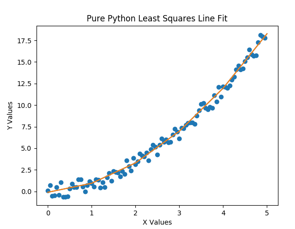 

Test Code 3

Now for a bit more of a challenge. We will use two input variables (i.e. X is now n \times 2 instead of n \times 1) and pass this two dimensional X through our two polynomial feature tools and perform essentially the same steps with the same types of sections, but now we will have a 3D output graph. Here’s the code from LeastSquaresPolyPractice_3b.py

import LinearAlgebraPurePython as la 
import MachineLearningPurePy as ml

from sklearn.linear_model import LinearRegression
from sklearn.preprocessing import PolynomialFeatures
import numpy as np

import matplotlib.pyplot as plt
from mpl_toolkits.mplot3d import Axes3D

import random
import sys

# Section 1: Fake data preparation 
#   and visualization
X = [[x/12 for x in range(2,102)],
     [2**(x/12) for x in range(0,100)]]

def y_of_x(xa):
    variation = random.uniform(-(xa[0]+xa[1])/4,(xa[0]+xa[1])/4)
    return 0.2*xa[0]**2 + 0.03*xa[0]*xa[1] + 0.7*xa[0] + 0.002*xa[1]**2 \
            + 0.04*xa[1] + 2.0 + variation
Y = []
for xa in la.transpose(X):
    Y.append(y_of_x(xa))

fig = plt.figure()
ax = plt.axes(projection='3d')
ax.scatter3D(X[0], X[1], Y)

# Section 2: Get fake data in correct format
X = la.transpose(X)
Y = la.transpose([Y])

# Section 3: Pure Python Tools Fit
poly_pp = ml.Poly_Features_Pure_Py(order=2) #, include_bias=False) # print(X) sys.exit()
Xpp = poly_pp.fit_transform(X)
ls_pp = ml.Least_Squares(add_ones_column=False)
ls_pp.fit(Xpp, Y)

# Section 4: SciKit Learn Fit
poly_sk = PolynomialFeatures(degree = 2)
Xps = poly_sk.fit_transform(X)
ls_sk = LinearRegression()
ls_sk.fit(Xps, Y)

# Section 5: Coefficients Comparison
tmp_ls_pp_coefs = sorted(ls_pp.coefs) # ls_pp.coefs # sorted(ls_pp.coefs)
rounded_ls_pp_coefs = [round(x,8)+0 for x in la.transpose(tmp_ls_pp_coefs)[0]] # 
print('PurePy  LS coefficients:', rounded_ls_pp_coefs)

tmp_ls_sk_coefs = ls_sk.intercept_.tolist() + ls_sk.coef_[0][1:].tolist()
tmp_ls_sk_coefs = sorted(tmp_ls_sk_coefs)
rounded_ls_sk_coefs = [round(x,8)+0 for x in tmp_ls_sk_coefs] # 
print('SKLearn LS coefficients:', rounded_ls_sk_coefs)

print('Coef Deltas:', [rounded_ls_pp_coefs[i] - rounded_ls_sk_coefs[i] 
        for i in range(len(rounded_ls_pp_coefs))])

# Section 6: Create Fake Test Data
XLS = [[x/12 for x in range(2,100,6)],
     [2**(x/12) for x in range(0,100,6)]]

# Section 6.1: Predict with Fake Test Data
#   Using Pure Python Tools
XLSpp = poly_pp.transform(la.transpose(XLS))       
YLSpp = ls_pp.predict(XLSpp)
YLSpp = la.transpose(YLSpp)[0]

# Section 6.2: Predict with Fake Test Data
#   Using SciKit Learn Tools
XLSsk = poly_sk.transform(la.transpose(XLS))
YLSsk = ls_sk.predict(XLSsk)
YLSsk = YLSsk.tolist()
YLSsk = la.transpose(YLSsk)[0]

# Section 7: Calculate Prediction Differences 
YLSpp.sort()
YLSsk.sort()
deltas = [ YLSpp[i] - YLSsk[i] for i in range(len(YLSpp)) ]
print( '\nPrediction Deltas:', deltas , '\n')

# Section 8: Plot Both Methods
ax.plot3D(XLS[0], XLS[1], YLSpp)
ax.plot3D(XLS[0], XLS[1], YLSsk)
ax.set_xlabel('X0 Values')
ax.set_ylabel('X1 Values')
ax.set_zlabel('Y Values')
ax.set_title('Pure Python Least Squares Fit with Two 2nd Order Inputs')
plt.show()

The output from the above code is shown below along with its 3D output graph. As before, the two tool sets, pure python and scikit learn, have extremely small prediction deltas and the two graph lines, that run through the initial fake data points, follow the same path. The sorted coefficients are identical (once rounded off). AGAIN, WITH NO RANDOM NOISE injected into the outputs, the coefficients would exactly match the initial coefficients. If you run the 3a version of the file, you will see this.

PurePy  LS coefficients: [-6.08262817, -2.54019522, -0.82948869, 
                           0.00555883, 1.45111668, 6.80215289]
SKLearn LS coefficients: [-6.08262817, -2.54019522, -0.82948869, 
                           0.00555883, 1.45111668, 6.80215289]
Coef Deltas: [0.0, 0.0, 0.0, 0.0, 0.0, 0.0]

Prediction Deltas: [1.2529532966709667e-10, 2.403943710760359e-11, -3.4301450568818836e-11, -5.644729128562176e-11, -5.043787609793071e-11, -2.5627500122027413e-11, 7.579714633720869e-12, 3.83000298143088e-11, 5.629097188375454e-11, 5.374722888973338e-11, 2.800959464366315e-11, -1.510613856225973e-11, -5.782396783615695e-11, -7.152323178161168e-11, -2.665956344571896e-11, 6.485834092018194e-11, 4.3939962779404595e-11]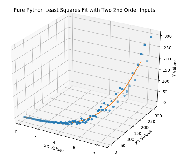 

A Cool Finding

While creating the fake data for these test files, I “brilliantly” created collinear data for the two inputs of X. This resulted in the pure python tools generating different coefficients than those created by the scikit learn tools, and I lost some hair over this. However, once I removed the collinearity between the X inputs, the coefficients matched exactly (or within a reasonable tolerance). After much reflection (i.e. thinking it over during an extra long hot shower), I felt that I could honestly say that I liked the way the pure tools reacted to collinearity more. With the pure tools, the coefficients with one of the collinear variables were 0.0. I’d prefer to detect collinearity with preprocessing tools, but this was a pleasant surprise.

Closing

If you’ve gone through every blog up until now, I am hoping, even trusting, that you are beginning to find the value to what we are doing and how we go about it. If not, I hope you will hang in there, because this approach of math theory all the way to code without relying on modules should help us to continue to grow our insights. I’d like to tell you what the next post will be, but I have a confession to make about that. My biggest stress by far in growing this blog is the order of posts. I would like to go through the perfect detail in the perfect order, but realistically speaking, I will probably have to back track some even if I work VERY hard to determine the best order of posts. I have about 10 posts in the works, and I am struggling to decide on which one to do next. Regardless, I hope to post again soon.

Until next time …