Find the files on GitHub

Overview

We now take a new, necessary, and important direction change to training our mathematical machines (i.e. models). Up to this point in the blog posts, we have used direct, or closed form, mathematical solutions such as those found in linear algebra. As usual, with these types of posts, we will start from concepts that lead us to the math and then code up the math step by step in python without using numpy or scipy. As always, we do this to understand principles of data science, machine learning and artificial intelligence better, and not because we do not love and appreciate numpy, scipy, and all the other great python modules out there in the wild. As always, do try to read as little as possible before you start trying to derive the math and code it up on your own. Then, compare to what is here. However, if you need to read all of it, no judgement.

Background of Gradient Descent

By analogy, if closed form solutions were a person named Math, we’d ask Math a question, and Math would give us a direct answer. “Hey Math, I have this data, and I want to know the best place in this model’s parameter space (the weights for the model) that will give the best predictions. Can you tell me?” Math gives us a direct answer telling us exactly where in the model’s parameter space we should be to make the best possible predictions. Previous posts have used this type of Math.

Some numerical techniques prevent a complete reliance on linear algebra solving techniques or closed form solutions. When mathematical situations such as these arise, we turn to gradient descent. Gradient descent is simple yet requires tools and thinking distinct from those belonging to the realm of closed form solutions. Gradient descent is math, but let’s say that gradient descent is a different type of math named Explorer. When we ask Explorer a question. Explorer doesn’t answer us with a direct answer. It may seem like a direct answer, given the speed of modern computers, but it’s not. Explorer goes on a journey taking many steps through a model’s error space along paths of maximum error reducing gradients (i.e. slopes) of

\dfrac {error \enspace change}{parameter \enspace change}

until Explorer arrives at a point in that error space that “seems” to be the smallest. Stepping along the current maximum gradient with an appropriately sized step is important. There are times when Explorer can be in a region of the parameter space that seems to have the lowest error when there can actually be a smaller error elsewhere in the overall (global) parameter space. In such cases, we can employ methods that help Explorer find these global minimums. However, for now, and because most problems we will encounter have a local minimum that is also a global minimum, let’s focus on the math around basic gradient descent and the code to implement that math. In later posts, we will discuss more ways to help Explorer (gradient descent techniques) increase the likelihood of finding the global minimums when multiple local minimums exist. If this explanation seems lacking or confusing, I encourage you to also read “An analogy for understanding gradient descent” on this Wikipedia Page. It’s always good to learn from multiple references.

Baron Augustin-Louis Cauchy made many great contributions to mathematical techniques supportive of engineering and physics. He originated the use of gradient descent as a solution method. Thank you Baron Cauchy! Let’s explore in more detail what gradient descent is, why we need it, and how to use it.

The term gradient may be familiar to you as the inclination of a road or path of some kind (i.e. a slope). In physics, it is an increase / decrease in a property from one point in space, or time, to the next. We, as data scientists, care about the gradient of a model’s predictive errors. Gradient(s) of the error(s) are with respect to changes in the model’s parameter(s). We want to descend down that error gradient, or slope, to a location in the parameter space where the lowest error(s) exist(s). To mathematically determine gradient(s), we differentiate a cost function. A cost function can also be referred to as an error function, a loss function, and even sometimes as an objective function. I wish our data science terms were in less flux, but our field is exploding with growth, and we have some variations in terminology due to the influx of great talent from many technical fields.

The Math

What is a cost function? It’s a function that calculates our model’s predictive errors, and it is of the form of equation 1 below. The term y_{act} refers to the actual output data, or labels, from the data that will be used to train our mathematical machines or models, and the term y_{pred} refers to the predictions from those models that are at a given state in their training.

\tag{1} E = (y_{pred} - y_{act})^2 \tag{1.1} y_{pred} = m x + b \tag{1.2} E = ((m x + b) - y_{act})^2 = \Delta^2

There can be many corresponding values for y_{act} and x. We typically want to use most of these values for training and hold some back for testing. Since we are focusing on gradient descent, we will not do this in this post. We will illustrate this split of training and testing data thoroughly in later posts.

At this point, I want to stress what I feel is an important philosophy of math type thought with respect to our cost function. With real world data that has noise and variance and does not follow an exact mathematical function (e.g. the most common case), we are searching for (seeking to move toward) the best predictions and not some function that will pass exactly through each of our training values. Also, when performing basic math to determine the slope of a line, we subtract a previous y (output) value from a current y value and divide that change in y by a corresponding change in x (the subtraction of a previous x (input) value from a current x value). In other words, we are quantitatively describing where we are going from where we were. In the cost function, we want to quantitatively describe where we want to go with respect to where we were (i.e. to predictions from messy real world training data). That’s why we have

\Delta = ((m x + b) - y_{act})

“But Thom! Why worry about this when we are going to square that difference?” Because, we are also about to take the derivative of the square of that difference, which will give us a slope of the cost function with respect to corresponding changes in model parameters, and the sign can flip depending on order of subtraction. It is good to know why we would subtract the actual values from the predicted ones, so that we have confidence and consistency in what signs that we choose to use in the math below.

Why is our error function called a cost function? Researching the history of word usage is hard, but, in this case, it’s valuable to at least think about why it’s good to call it a cost function. Mispredicting an output is costly. Not making any prediction at all is even more costly! Thus, we do the best that we can to minimize the cost and maximize the profit from our predictive modeling efforts. To obtain the mathematical gradient(s) needed, we apply differential principles of Calculus on our cost function. Again, our solution technique uses gradient calculations to find directions that we should take as we take small steps through a model’s parameter space. Each step reduces our cost (and increases our modeling profit) a little bit. We keep taking small steps until we “mathematically” sense that we are at a minimum error. Equations 2 show us the calculus steps for finding the gradient (slope) for the equation of a line. HOWEVER, remember, differentiation is an analytical determination of the gradient (i.e. slope) of a function at any given set of inputs. IF EVER NECESSARY, we could numerically differentiate a function at different inputs. It’s always good to remain aware of the concepts being employed.

\tag{2.1} \dfrac {\partial E}{\partial m} = \dfrac {\partial E}{\partial y_{pred}} \dfrac {\partial y_{pred}}{\partial m} \tag{2.2} \dfrac {\partial E}{\partial y_{pred}} = 2 ((m x + b) - y_{act}) \tag{2.3} \Delta = ((m x + b) - y_{act}) \tag{2.4} \dfrac {\partial y_{pred}}{\partial m} = x \tag{2.5} \dfrac {\partial E}{\partial m} = 2 x \Delta

Following similar steps to the above, the gradient \dfrac {\partial E}{\partial b} that guides us to the lowest error for b is shown in equation 3.

\tag{3} \dfrac {\partial E}{\partial b} = 2 \Delta

Now we have an equation to calculate gradients at any point in our model’s parameter space. How do we take the small steps through that space using these gradient calculations? We use the method shown in equation 4 below.

\tag{4} m = m - LR \cdot ( x \cdot \Delta) \\ b = b - LR \cdot ( \Delta)

Please note that LR is a small value, and we have allowed the 2 from our derivatives to be absorbed into LR.

The negative sign in equations 4 is due to the calculus and algebra steps that we took to find the gradient and apply it to our gradient descent equation. We wish to go to a point where our cost function gradient is zero. If we were performing some type of maximization for a function other than a cost function that was a high point in that functions space with respect to model parameters, the calculus and algebra for finding the gradient and using gradient descent would take us to that maximum. Thus, the descent part is a bit of a misnomer. Gradient descent / ascent takes us to a place where a given function has zero slope. However, this math is often applied to cost function minimization, so we usually do descend to a low point of a mathematical valley.

The general form for updating any weight w of a model using derivatives of a cost function that we wish to minimize is shown in equation 5.

\tag{5} w = w - LR \cdot \dfrac {\partial E}{\partial w}

A Toy Example of Math to Code

This section is meant to explain why I present the progression of coding like I have done below. I am a big fan of starting with stupid simple code examples to get going on a new project or to gain some momentum on how to employ a new methodology. I’ve seen this help others that I’ve mentored, and I trust it will help you too. It’s also a great way to get into coding flow. This stage is only meant as a way to “work out” concepts until you prove to yourself “I’ve got it!” It’s also a great idea to keep your own directory of such concept code learning. This way, you have a host of simple conceptual code to refer back to as needed. This also allows leaner development. You can try new things and test them outside your larger applications until you are ready to pull them into one of your larger applications. This also helps you to think more modular and to make good reusable code. The upcoming sections presents such a coding approach to an extent.

Even though I am a big fan of the approach that I’ve just explained, I am a bigger fan of object oriented programming. To me, classes are like miniature containers. They group data structures and methods together. Each method can be made to do ONE specific thing, which makes code easier to read and maintain. As the architect of your classes, you determine the inputs and outputs to the class. You decide what data and methods are for “internal use only”. In case you are somewhat new to classes, I hope that you will keep such things in mind as you look through the code below.

Basic Concept Code for Modeling a Line

Remember, this code is on GitHub. I hope you’ve already cloned or downloaded it and are running this code as you read. The code below is from GradDesc1.py in the repo.

from Plot_Tools import Basic_Plot as BP
import random
import sys

# Section 1: Fake Training Data Preparation
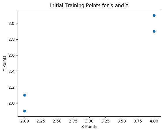
Xp = [2, 2, 4, 4]
X = [[1, x] for x in Xp]
Y = [2.1, 1.9, 3.1, 2.9]
BP(xp=Xp, yp=Y,
   t='Initial Training Points for X and Y')

# Section 2: Solution of Model Parameters / Weights
b = 0.01  # initial value for y-intercept
m = 0.025  # initial value for slope
Yp = [0, 0, 0, 0]
LR = 0.001

cost_list = []
b_list = []
m_list = []

num_pts = len(X)
for it in range(100000):
    for i in range(num_pts):
        # Prediction based on current weights
        Yp[i] = X[i][0] * b + X[i][1] * m

        # Error based on current weights
        delta = Yp[i] - Y[i]
        cost = delta ** 2.0

        # The gradients for y-intercept and slope
        db = X[i][0] * delta
        dm = X[i][1] * delta

        # Update the weights
        b = b - LR * db
        m = m - LR * dm

    if it % 100 == 0:
        cost_list.append(cost)
        b_list.append(b)
        m_list.append(m)

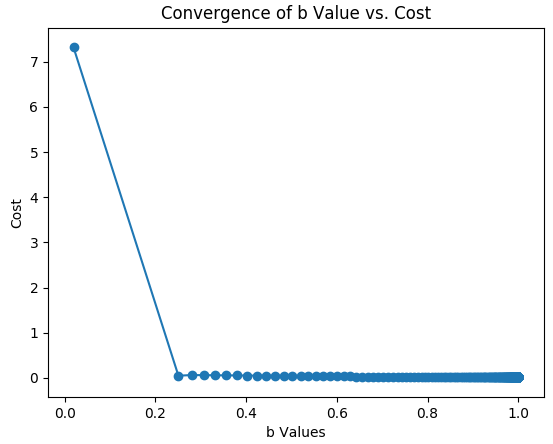
# Section 3: Show convergence of weights
BP(x=b_list, y=cost_list,
   t='Convergence of b Values vs. Cost',
   x_t='b Values', y_t='Cost',
   xp=b_list, yp=cost_list)

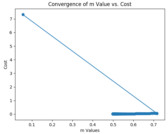
BP(m_list, cost_list,
   t='Convergence of m Values vs. Cost',
   x_t='m Values', y_t='Cost',
   xp=m_list, yp=cost_list)

# Section 4: Create Fake Test Data
Xtp = [x/20.0 for x in list(range(100))]
Xtc = [[1, x] for x in Xtp]
Yt = []

# Section 5: Predictions Using Fake Test Data
for x in Xtc:
    yt = b * x[0] + m * x[1]
    Yt.append(yt)

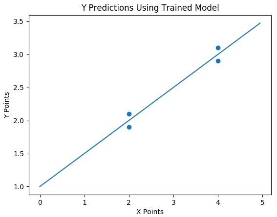
BP(x=Xtp, y=Yt,
   t='Y Predictions for X from Trained Model',
   xp=Xp, yp=Y)

In the imports, you will notice the import of Basic_Plot from Plot_Tools. Plot_Tools is a file in the repo for this post that houses the function Basic_Plot. To reduce writing similar lines over and over for plotting, it seemed best to make a function for those standard plots.

Section 1 simply creates our fake training data. Note the list comprehension of X = [[1, x] for x in Xp] that adds 1‘s to the first column of X. These 1‘s are for the bias term (y-intercept), and how they are used in the code will become more apparent as we move through this post in case you have not read the previous posts of this blog. A plot of our over simplified training data is shown below in figure 1.

Section 2 performs the actual solution through small steps using the gradients for b (the y-intercept of the line) and m (the slope of the line). Note that we first initialize values outside the solution loop and then instantiate some lists to hold values during the many steps of the solution. Next we enter the loop and for each input (x) and (output) y pair from the training data we:

1. have the model make a prediction using the current weights (i.e. the current values of b and m);
2. subtract the actual outputs from this prediction;
3. use the difference from step 2 to calculate the cost;
4. use the difference from step 2 to calculate gradients for b and m;
5. use the gradients and the learning rate (LR) to update b and m (our weights).

When we start the next iteration of the loop, we are calculating a prediction with updated weights (i.e. updated values for b and m). If we’ve stepped in the right direction, the output of the cost function will be less than the first calculation. If we have stepped in the wrong direction for some reason, it is possible that we will step toward an overflow error (and this can happen quite quickly if your cost function is not bound in some way!). Then we store values we wish to store for subsequent plotting. In case you’ve never seen something like if it % 100 == 0:, the % operator (modulus) in python simply returns the remainder when dividing a by b when you code a % b. We only want to store our values to our lists every 100 it steps (and of course you can change 100 to your storage interval liking).

Section 3 handles plotting the paths of our gradient descent solutions for b and m, which are shown below.

Finally, in Sections 4 and 5 we use the weights (b and m) obtained through the gradient descent method to make predictions using fake test data to see how well the predictions pass through our training data.

If you’re thinking the same thing that I am thinking, you’re thinking that the solution paths for b and m look a little strange. I would agree. It’s not that they are wrong; it’s just that they don’t look classy. After some exploration, I realized why they do that. The zigzag with m is due to the initial big correction from the gradient making it’s first big jump. Both look strange also due to the initial big jump. The path of travel for each weight also affects the path of the other weight. That is, we are simply looking at a lot of interactive solution dynamics. The communication interval is also hiding some things. Thus, I made a specific script to illustrate a solution path with respect to a cost function more clearly, and it is named Param_Sweep.py. It’s contents are below.

from Plot_Tools import Basic_Plot as BP
import random
import sys

# Section 1: Fake Training Data Preparation
Xp = [4]
X = [[1, x] for x in Xp]
Y = 3

# Section 2: Solution of Model Parameters / Weights
b = 1.0  # Fixed value for y-intercept - testing
m = 0.0  # initial value for slope
LR = 0.0001  # smaller learning rate for illustration

cost_list = []
m_list = []

num_pts = len(X)
for it in range(10000):
    Yp = X[0][0] * b + X[0][1] * m
    delta = Yp - Y
    cost = delta ** 2.0
    dm = X[0][1] * delta
    m = m - LR * dm
    if it % 50 == 0:
        cost_list.append(cost)
        m_list.append(m)  # b_list.append(m)

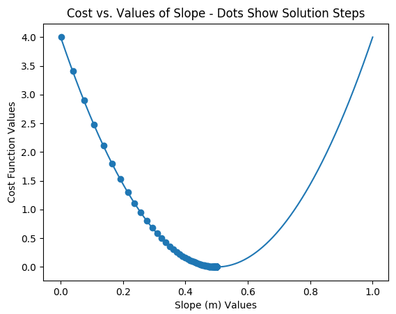
# SPECIAL SECTION: Parameter sweep plot of m vs. cost
sweep_m_list = []
sweep_cost_list = []

# sweep of slope vs. cost
for val in range(0, 10001):
    slope = val / 10000.0
    cost = ((b + X[0][1] * slope) - Y) ** 2.0

    sweep_m_list.append(slope)
    sweep_cost_list.append(cost)

BP(x=sweep_m_list, y=sweep_cost_list,
   xp=m_list, yp=cost_list,
   t='Cost vs. Values of Slope - Dots Show Solution Steps',
   x_t='Slope (m) Values', y_t='Cost Function Values')

The script above creates a line plot first of cost given a sweep of values for m from 0 to 1. Then it uses gradient descent to only solve for m and uses only one training point. This is ONLY for the purpose of illustrating gradient descent more clearly with respect to a cost function. The learning rate, the number of steps, and the communication interval are too small for practical purposes.

Moving Operations to Functions

To reiterate, the above code was simply used to “prove out our methods” before putting them into a more general, reusable, maintainable format. Let’s take the code above from GradDesc1.py and move it to individual functions that each perform separate portions of our gradient descent procedure. All of the code pieces for this section are contained in GradDesc2.py. I hope you will have it open, run it, and change it to your liking as you read.

We need the following functions:

1. a function for our model that will predict an output based on an input or set of inputs;
2. a function to calculate the difference between our predictions and our actual values;
3. a function to update our weights;
4. a function to perform gradient descent;
5. other nice functions to have would be:
   a) a function to calculate our cost, and
   b) a function to control recording / reporting frequency.

Code that will handle functionality 1 above for our model is shown in the following code block. Note how we are using the dimensions of X to obtain the number of iterations needed for each of the for loops. We also make sure that all records of X have the same number of dimensions. For each record of X, we obtain one predicted output. The predicted output is built up over the number of dimensions using the inner for loop. This way we can have a flexible number of dimensions, which our function can discern from the number of elements in each record of X.

def model(X, w):
    records = len(X)
    Yp = [0] * records
    dims = len(X[0])

    dim_chk = sum([dims == len(xi) for xi in X]) == records
    assert dim_chk, 'NOT ALL X RECORDS HAVE SAME DIMENSIONS'

    for i in range(records):
        for j in range(dims):
            Yp[i] += X[i][j] * w[j]

    return Yp

Code that will handle functionality 2 above for calculating the differences between predicted and actual output values is shown in the next code block. Note again how we use the dimensions of the X array to obtain information needed by the for loop and to construct delta.

def delta_calc(Yp, Y):
    records = len(X)
    delta = [0] * records

    for i in range(records):
        delta[i] = Yp[i] - Y[i]

    return delta

Code that will handle functionality 3 from the above is shown in the next code block. Much like the previous 2 functions above, information about the X array is used to gather more needed information. Note the negative sign in front of the learning rate (LR) for gradient “descent”.

def update_weights(w, delta, X, LR):
    records = len(X)
    dims = len(X[0])

    for i in range(records):
        for j in range(dims):
            w[j] = w[j] - LR * X[i][j] * delta[i]

    return w

Now, we need to bring these functions together into a series of operations that will perform gradient descent, providing functionality 4 called out above, in a loop until the solution reaches a desired tolerance. Code that can achieve these aims is shown below.

def solver(X, w, Y, LR, ci,
           tol=1.0e-16, max_cnt=1e9):

    cost_delta = 1.0
    cost_last = 1.0
    cnt = 0
    cost_list = []
    cnt_list = []
    w_list = []

    while cost_delta > tol:
        Yp = model(X, w)
        delta = delta_calc(Yp, Y)
        w = update_weights(w, delta, X, LR)

        cost_now = cost(delta)
        cost_delta = abs(cost_last - cost_now)
        cost_last = cost_now

        if record_value(cnt, ci):
            cost_list.append(cost_now)
            cnt_list.append(cnt)
            w_list.append(w.copy())

        cnt += 1

        if cnt > max_cnt:
            print("Exiting Due To Exceeding Max Iterations")
            break

    return w, cost_list, delta, cnt, cnt_list, w_list

Note that all the functions needed for a single step of the gradient descent procedure are accomplished by the first three lines inside the while loop, and each of those lines is calling the three functions that were just previously described. The while loop that checks for a given tolerance of convergence is an upgrade from the for loop that used a fixed number of iterations that we were required to set. All other lines in this function serve various preparation, recording and status checking operations. In the next three lines, we

1. find the current value of the cost function as cost_now using a function that we haven’t shown yet that calculates the cost using the cost function described above,
2. subtract cost_now from the last value (cost_last that had to be initialized before the while loop as you see) to obtain cost_delta, and then
3. make sure we update cost_last with cost_now for the next iteration.

When cost_delta is less than our tolerance, the while loop will exit. Until the while loop is exited, we are recording, when allowed by the record_value function that returns True when a communication interval has been met, values for cost (cost_now), iteration counts (cnt), and weights (w). Note the appending of w.copy() to the w_list. If you don’t do this, because w is being updated each loop, the whole list will contain the final weights. Finally, if we’ve looped an insane number of times, and cnt > max_cnt, break out of the while loop. It’s always a good idea to have a safeguard like this when using while loops in my opinion.

The final two functions that were mentioned above in the previous code block, but were not yet shown, are now presented below.

def cost(delta):
    total_cost = 0
    for value in delta:
        total_cost += value ** 2

    return total_cost


def record_value(count, comm_interval):
    if count % comm_interval == 0:
        return True
    else:
        return False

Again, all of these functions are contained in GradDesc2.py in the repo along with the code below that uses those functions to perform what we’ve previously done in GradDesc1.py. I hope you are running it and refactoring it to your liking.

# Section 1: Fake Training Data Preparation
Xp = [2, 2, 4, 4]
X = [[1, x] for x in Xp]
Y = [2.1, 1.9, 3.1, 2.9]
ws = [random.random()] * len(X[0])
LR = 0.01

# Section 2: Solve / train
ws, cost_list, delta, cnt, cnt_list, w_list = \
    solver(X, ws, Y, LR, 1)

# Section 3: Report training results
print(f'Delta = {delta}, Count = {cnt}')
ws = [round(x, 6) for x in ws]
print(f'Solved Weights: {ws}')

BP(cnt_list, cost_list,
   t='cost vs. Step', x_t='Step', y_t='cost')

# Plot learning path of weights
for i in range(len(ws)):
    wi_list = [pair[i] for pair in w_list]
    title = f'Cost vs Weight {i}'
    x_t = f'Weight {i}'
    y_t = 'Cost'
    BP(wi_list, cost_list,
       t=title, x_t=x_t, y_t=y_t)

# Section 4: Fake test data creation and predictions
Xtp = [x/20.0 for x in list(range(100))]
Xtc = [[1, x] for x in Xtp]
YtP = model(Xtc, ws)

BP(Xtp, YtP, xp=Xp, yp=Y,
   t='Predictions vs. Fake X',
   x_t='Fake X', y_t='Predicted Y')

Since the code above is much like operations previously described, I will leave it to our readers to look through it and modify it for further exploration and learning. Note that the communication interval is set to “1” only to provide more visibility to the solution progress. If you wish to see more such detail, experiment with changing the learning rate (LR) to smaller numbers.

Functions to Class

Let’s turn our set of functions into a reusable class that we can store in a toolbox for later instantiation on different problems. The file for our new class in the post repo is Gradient_Descent_Solver.py, and it is shown below. Descriptions of the various data structures and methods are below the code block for the class.

from Plot_Tools import Basic_Plot as BP
import random


class Gradient_Descent_Solver:
    def __init__(self, X, Y, LR,
                 ci=1000, tol=1e-12,
                 max_cnt=1e9, rnd=6):
        self.X = X
        self.Y = Y
        self.LR = LR
        self.ci = ci
        self.tol = tol
        self.max_cnt = max_cnt
        self.rnd = rnd

        self.num_records = len(X)
        self.num_dims = len(X[0])

        self.Yp = [0] * self.num_records
        self.delta = [0] * self.num_records
        self.randomize_weights()

        self.cnt_list = []
        self.cost_list = []

    def set_weights(self, ws):
        self.ws = ws

    def set_labels(self, Y):
        self.Y = Y

    def randomize_weights(self):
        self.ws = [random.random()] * self.num_dims

    def model(self, X):
        num_records = len(X)
        self.Yp = [0] * num_records

        for i in range(num_records):
            for j in range(self.num_dims):
                self.Yp[i] += X[i][j] * self.ws[j]

        return self.Yp

    def train(self):
        cost_delta = 1.0
        cost_last = 1.0

        self.count = 0
        self.cost_list = []
        self.cnt_list = []

        while cost_delta > self.tol and self.__iterations_below_max__():
            self.model(self.X)
            self.__update_weights__()

            self.cost_now = self.__cost__()
            cost_delta = abs(cost_last - self.cost_now)
            cost_last = self.cost_now

            self.__record_values__()

    def __update_weights__(self):
        for i in range(self.num_records):
            self.delta[i] = self.Yp[i] - self.Y[i]
            for j in range(self.num_dims):
                self.ws[j] = \
                    self.ws[j] - self.LR * self.X[i][j] * self.delta[i]

    def __cost__(self):
        total_cost = 0
        for value in self.delta:
            total_cost += value ** 2

        return total_cost ** 0.5

    def __record_values__(self):
        self.count += 1

        if self.count % self.ci == 0:
            self.cost_list.append(self.cost_now)
            self.cnt_list.append(self.count)

    def __iterations_below_max__(self):
        if self.count < self.max_cnt:
            return True
        else:
            print("Exceeded Max Iterations")
            return False

    def report_results(self):
        ws = [round(x, 6) for x in self.ws]
        print(f'Solved Weights: {ws}')
        print(f'Iteration Steps to Solution: {self.count}')

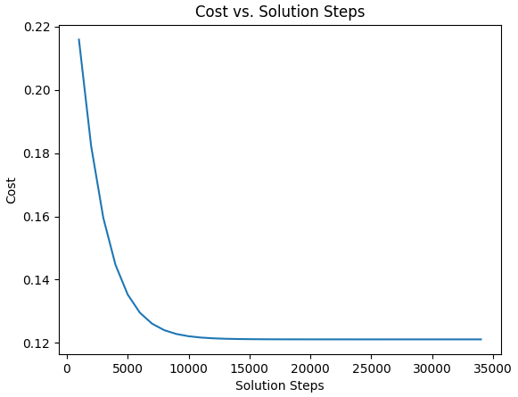
    def plot_solution_convergence(self):
        BP(self.cnt_list, self.cost_list,
           t='Cost vs. Solution Steps',
           x_t='Solution Steps', y_t='Cost')

    def plot_predictions(self, X, Y, col_of_X=1):
        Xsp = [row[col_of_X] for row in self.X]
        Xtp = [row[col_of_X] for row in X]
        BP(Xtp, self.Yp, xp=Xsp, yp=self.Y,
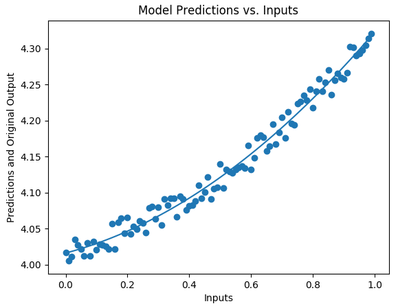
           t='Model Predictions vs. Inputs',
           x_t='Inputs',
           y_t='Predictions and Original Output')

Let’s now talk through each of the methods above. Please note that when a function is named with double underscores at the beginning and end, such as __function_name__, that function is intended to be private to the class. Any function with out pre and post “__” are meant to be interfaces to the class.

1. __init__ only requires X and Y training data, and a learning rate (LR). There are four other parameters that have defaults:
   ci is the communication interval as previously explained,
   tol is the tolerance cost changes as used in GradDesc2.py,
   max_cnt is our safety break as used in GradDesc2.py,
   rnd is to round off the reporting of our weights.
   Also as before, we use dimensions of the X array to obtain the number of records and the number of dimensions for our model. We:
   a) create place holders for our output predictions,
   b) our deltas between predicted and actual outputs,
   c) initialize our weights with random values, and
   d) instantiate lists to hold values that we care to know.
2. set_weights allows us to set the weights at any point in time for times where we might want to use the model without using the trained weights.
3. set_labels allows us to independently reset the training weights in case we would want to.
4. randomize_weights, which we saw called in the init function, simply sets the weights for the class with random values.
5. model does what we’ve seen previously. It simply uses the current weights to make an output prediction.
6. train is pretty much like solve from GradDesc2.py. Efforts have been made to increase it’s elegance. The deltas calculation happens directly in __update_weights__ now, and all logic to break out of the while loop is in line with the while statement with a method call to ensure counts are less than the max. The values to be recorded are placed in the __record_values__ method.
7. __update_weights__ is the same, except, as already stated, we’ve added the deltas calculations to this method.
8. __cost__ is the cost function and simply uses the current deltas.
9. __record_values__ keeps the count of the gradient descent steps and controls the frequency of communications / values recording.
10. __iterations_below_max__ simply returns a Boolean as to whether or not the gradient descent steps are below the max counts.
11. report_results, plot_solution_convergence, and plot_predictions will be considered self explained based on their code and previous similar operations.

More Testing of Our Work

It’s time to have some fun with our new class, or your hacked up improved version of what’s been presented so far. There are four testing files named Testing_#.py. We will leave you to explore 1 thru 3 on your own. Let’s go straight to Testing_4.py. The code for it is shown in the code block below. An explanation of the code and outputs follows the block.

import Gradient_Descent_Solver as GDS
import random

# #############################################################################
# Section 1: Create Fake X Data
it = [x/100 for x in list(range(100))]
X = [[x**0, x**1, x**2] for x in it]
wa = [4.0, 0.1, 0.2]


# Section 2: Create Fake Y Data
def Y_maker(X, w):
    Y = []
    for x in X:
        y = 0
        for i in range(len(w)):
            y += x[i] * wa[i]
        Y.append(y + y / 100 * random.random())

    return Y


Y = Y_maker(X, wa)

# # Section 3: Instantiate Our Class
LR = 0.001
gds = GDS.Gradient_Descent_Solver(X, Y, LR)

# Section 4: Train model and Show Results
gds.train()
gds.report_results()
gds.plot_solution_convergence()

# Section 5: Create Fake Test Inputs, Predict, Plot
it = [x/100 for x in list(range(100))]
Xt = [[x**0, x**1, x**2] for x in it]
Yt = gds.model(Xt)
gds.plot_predictions(Xt, Yt, col_of_X=1)

In Section 1, we cleverly make some good fake training inputs for a second order function and establish some made up weights in preparation for creating fake outputs. In Section 2, we define a function to make our fake training outputs with injected fake noise using our made up weights, and use that function to make those outputs. In Section 3, we initialize our LR and instantiate our gradient descent solver class. In Section 4, we train the model and report and plot the results of the training.

Outputs:
Solved Weights: [4.01627, 0.113287, 0.193621]
Iteration Steps to Solution: 34306

In Section 5, we create different fake test inputs, use our trained model to predict outputs, and plot those predictions through our original training data. The plot is shown below.

Hey Thom, I Noticed That …

Why didn’t I reuse my linear algebra functions that we developed together in previous posts? Not everyone coming here will read those posts first. I wanted this post to stand a bit on its own without requiring people new to IMLAI to go read that first. Plus, these posts are more educational in nature, so it’s best to let all steps be obvious. However, in our work as data scientists, YES, develop good tools and use them often (and even refactor them often).

Gradient Descent With Numpy

This section will not be a one liner or even a few lines. Let’s rebuild the class above (not completely) using numpy. The changes using numpy are quite elegant. It would be best to compare these two classes side by side. The new gradient descent class with numpy is in the repo in a file named, surprisingly, Gradient_Descent_Solver_with_Numpy.py.

from Plot_Tools import Basic_Plot as BP
import numpy as np
import sys


class Gradient_Descent_Solver_with_Numpy:
    def __init__(self, X, Y, LR,
                 ci=1000, tol=1e-12,
                 max_cnt=1e9, rnd=6):

        if type(X) is not np.ndarray:
            X = np.asarray(X)
        if type(Y) is not np.ndarray:
            Y = np.asarray(Y)

        self.X = X
        self.Y = Y
        self.LR = LR
        self.ci = ci
        self.tol = tol
        self.max_cnt = max_cnt
        self.rnd = rnd

        self.num_records = len(X)
        self.num_dims = len(X[0])

        self.Yp = np.zeros((self.num_records, 1))
        self.delta = np.zeros((self.num_records, 1))
        self.randomize_weights()

        self.cnt_list = []
        self.cost_list = []

    def set_weights(self, ws):
        if type(ws) is not np.ndarray:
            ws = np.asarray(ws)

        self.ws = ws

    def set_labels(self, Y):
        if Y is not np.ndarray:
            Y = np.asarray(Y)

        self.Y = Y

    def randomize_weights(self):
        self.ws = np.random.rand(self.num_dims, 1)

    def model(self, X):
        if X is not np.ndarray:
            X = np.asarray(X)
        self.Yp = np.matmul(X, self.ws)
        return self.Yp

    def train(self):
        cost_delta = 1.0
        cost_last = 1.0

        self.count = 0
        self.cost_list = []
        self.cnt_list = []

        while cost_delta > self.tol and self.__iterations_below_max__():
            self.model(self.X)
            self.__update_weights__()

            self.cost_now = self.__cost__()
            cost_delta = abs(cost_last - self.cost_now)
            cost_last = self.cost_now

            self.__record_values__()

    def __update_weights__(self):
        self.delta = self.Yp - self.Y
        dcdw = np.sum(self.X * self.delta, axis=0).reshape((self.num_dims, 1))
        self.ws = self.ws - self.LR * dcdw

    def __cost__(self):
        return np.sum(np.square(self.delta)) ** 0.5

    def __record_values__(self):
        self.count += 1

        if self.count % self.ci == 0:
            self.cost_list.append(self.cost_now)
            self.cnt_list.append(self.count)

    def __iterations_below_max__(self):
        if self.count < self.max_cnt:
            return True
        else:
            print("Exceeded Max Iterations")
            return False

    def report_results(self):
        ws = np.around(self.ws, decimals=6)
        print(f'Solved Weights: {ws}')
        print(f'Iteration Steps to Solution: {self.count}')

    def plot_solution_convergence(self):
        BP(self.cnt_list, self.cost_list,
           t='Cost vs. Solution Steps',
           x_t='Solution Steps', y_t='Cost')

    def plot_predictions(self, X, Y, col_of_X=1):
        if type(X) is not np.ndarray:
            X = np.asarray(X)
        Xsp = self.X[:, col_of_X].tolist()
        Xtp = X[:, col_of_X].tolist()

        BP(Xtp, self.Yp, xp=Xsp, yp=self.Y,
           t='Model Predictions vs. Inputs',
           x_t='Inputs',
           y_t='Predictions and Original Output')

Let’s go thru the methods and analyze the changes that were made for the numpy conversion.

1. __init__ If X or Y come in as non-numpy arrays, they are converted to numpy arrays. The initialization of self.Yp and self.delta are now accomplished with the numpy zeros function.
2. set_weights Convert ws to a numpy array if necessary and make the weights an attribute of the class.
3. set_labels Convert Y to a numpy array if necessary and make them an attribute of the class.
4. randomize_weights Use the numpy random class to create new starting weights, self.ws, with the correct dimensions.
5. model Wow! This is where it got elegant. A matrix multiplication of the inputs (X) and the weights (self.ws) to get the output given the current weights. Many people use the numpy dot method for matrix multiplication, and that’s a fine practice, but my simple brain prefers to use the more explicit (description wise) matmul method of numpy.
6. train Nothing new here. The changes happen in the methods that train calls.
7. __update_weights__ Where did all the code go?!?! We calculate the self.delta vector, and then we have a slick numpy one liner that calculates ALL the \dfrac {\partial E}{\partial w} ‘s, and this vector of partial derivatives is named dcdw in code, which stands for change in cost over change in weights. One liners are great when they are clear to you, but they’re frustrating when you don’t! The self.X * self.delta multiplies each row of self.X by the corresponding element in the column vector self.delta. The sum method sums each row of the result. Unfortunately, this summing operation does NOT retain the column vector shape, so we simply reshape it. Voila! One liner explained (I hope!). Finally, the last line does the gradient descent update of the weights.
8. __cost__ Square each element of self.delta, sum all those squares to one total, and take the square root of that total.
9. __record_values__ and __iterations_below_max__ and plot_solution_convergence are the same.
10. report_results uses the numpy around method to perform the rounding of the reported weights.
11. plot_predictions ensures that the X passed in is converted to numpy format if necessary and then uses the convenient column slicing tools of numpy arrays to capture the columns we want to plot our results against.

This class is instantiated and used in the files named Testing_#_np.py in the repo, where # has values of 1 thru 4. They all yield the same results as their Testing_#.py counterparts. I encourage you to look at each Testing_#_np.py and Testing_#.py pair side by side, especially number 4.

Closing and Next Steps

This post was preparatory for some upcoming posts. Gradient descent will be essential to the solving of many of the models that we will cover. I hope you were able to clone the repo and make some good explorations using the code. As always, please feel free to refactor things and make it your own. And to that last point, it really does pay in my opinion, to sit back and think about how to make code more elegant. I hope what you see in this and other posts gives you some ideas about how to make your own code better in every way. Until next time …