Get the files for this project on GitHub

Introduction

With the tools created in the previous posts (chronologically speaking), we’re finally at a point to discuss our first serious machine learning tool starting from the foundational linear algebra all the way to complete python code. Those previous posts were essential for this post and the upcoming posts. This blog’s work of exploring how to make the tools ourselves IS insightful for sure, BUT it also makes one appreciate all of those great open source machine learning tools out there for Python (and spark, and there’s ones for R of course, too). There’s a lot of good work and careful planning and extra code to support those great machine learning modules AND data visualization modules and tools. Let’s recap where we’ve come from (in order of need, but not in chronological order) to get to this point with our own tools:

1. BASIC Linear Algebra Tools in Pure Python without Numpy or Scipy
2. Find the Determinant of a Matrix with Pure Python without Numpy or Scipy
3. Simple Matrix Inversion in Pure Python without Numpy or Scipy
4. Solving a System of Equations in Pure Python without Numpy or Scipy

We’ll be using the tools developed in those posts, and the tools from those posts will make our coding work in this post quite minimal and easy. We’ll only need to add a small amount of extra tooling to complete the least squares machine learning tool. However, the math, depending on how deep you want to go, is substantial.

We will be going thru the derivation of least squares using 3 different approaches:

1. Single Input Linear Regression Using Calculus
2. Multiple Input Linear Regression Using Calculus
3. Multiple Input Linear Regression Using Linear Algebraic Principles

LibreOffice Math files (LibreOffice runs on Linux, Windows, and MacOS) are stored in the repo for this project with an odf extension. I hope that you find them useful. They store almost all of the equations for this section in them. Let’s start with single input linear regression

Single Input Linear Regression

If you know basic calculus rules such as partial derivatives and the chain rule, you can derive this on your own. As we go thru the math, see if you can complete the derivation on your own. If you get stuck, take a peek. If you work through the derivation and understand it without trying to do it on your own, no judgement. Understanding the derivation is still better than not seeking to understand it.

A simple and common real world example of linear regression would be Hooke’s law for coiled springs:

\tag{1.1} F=kx

If there were some other force in the mechanical circuit that was constant over time, we might instead have another term such as F_b that we could call the force bias.

\tag{1.2} F=kx+F_b

If we stretch the spring to integral values of our distance unit, we would have the following data points:

\tag{1.3} x=0, \,\,\,\,\, F = k \cdot 0 + F_b \\ x=1, \,\,\,\,\, F = k \cdot 1 + F_b \\ x=2, \,\,\,\,\, F = k \cdot 2 + F_b

Hooke’s law is essentially the equation of a line and is the application of linear regression to the data associated with force, spring displacement, and spring stiffness (spring stiffness is the inverse of spring compliance). Recall that the equation of a line is simply:

\tag{1.4} \hat y = m x + b

where \hat y is a prediction, m is the slope (ratio of the rise over the run), x is our single input variable, and b is the value crossed on the y-axis when x is zero.

The actual data points are x and y, and measured values for y will likely have small errors. The values of \hat y may not pass through many or any of the measured y values for each x. Therefore, we want to find a reliable way to find m and b that will cause our line equation to pass through the data points with as little error as possible. The error that we want to minimize is:

\tag{1.5} E=\sum_{i=1}^N \lparen y_i - \hat y_i \rparen ^ 2

This is why the method is called least squares. Our “objective” is to minimize the square errors. That is we want find a model that passes through the data with the least of the squares of the errors. Let’s substitute \hat y with mx_i+b and use calculus to reduce this error.

\tag{1.6} E=\sum_{i=1}^N \lparen y_i - \lparen mx_i+b \rparen \rparen ^ 2

Let’s consider the parts of the equation to the right of the summation separately for a moment.

\tag{1.7} a= \lparen y_i - \lparen mx_i+b \rparen \rparen ^ 2

Now let’s use the chain rule on E using a also.

\tag{1.8} \frac{\partial E}{\partial a} = 2 \sum_{i=1}^N \lparen y_i - \lparen mx_i+b \rparen \rparen \tag{1.9} \frac{\partial a}{\partial m} = -x_i

Applying the chain rule, the result is

\tag{1.10} \frac{\partial E}{\partial m} = \frac{\partial E}{\partial a} \frac{\partial a}{\partial m} = 2 \sum_{i=1}^N \lparen y_i - \lparen mx_i+b \rparen \rparen \lparen -x_i \rparen)

Now we do similar steps for \frac{\partial E}{\partial b} by applying the chain rule.

\tag{1.11} \frac{\partial a}{\partial b} = -1

Using equation 1.8 again along with equation 1.11, we obtain equation 1.12

\tag{1.12} \frac{\partial E}{\partial b} = \frac{\partial E}{\partial a} \frac{\partial a}{\partial b} = 2 \sum_{i=1}^N \lparen y_i - \lparen mx_i+b \rparen \rparen \lparen -1 \rparen)

Now we want to find a solution for m and b that minimizes the error defined by equations 1.5 and 1.6. These errors will be minimized when the partial derivatives in equations 1.10 and 1.12 are “0”.

Let’s find the minimal error for \frac{\partial E}{\partial m} first. Setting equation 1.10 to 0 gives

0 = 2 \sum_{i=1}^N \lparen y_i - \lparen mx_i+b \rparen \rparen \lparen -x_i \rparen) 0 = \sum_{i=1}^N \lparen -y_i x_i + m x_i^2 + b x_i \rparen) 0 = \sum_{i=1}^N -y_i x_i + \sum_{i=1}^N m x_i^2 + \sum_{i=1}^N b x_i \tag{1.13} \sum_{i=1}^N y_i x_i = \sum_{i=1}^N m x_i^2 + \sum_{i=1}^N b x_i

Let’s do similar steps for \frac{\partial E}{\partial b} by setting equation 1.12 to “0”.

0 = 2 \sum_{i=1}^N \lparen -y_i + \lparen mx_i+b \rparen \rparen 0 = \sum_{i=1}^N -y_i + m \sum_{i=1}^N x_i + b \sum_{i=1} 1 \tag{1.14} \sum_{i=1}^N y_i = m \sum_{i=1}^N x_i + N b

Starting from equations 1.13 and 1.14, let’s make some substitutions to make our algebraic lives easier. The only variables that we must keep visible after these substitutions are m and b.

T = \sum_{i=1}^N x_i^2, \,\,\, U = \sum_{i=1}^N x_i, \,\,\, V = \sum_{i=1}^N y_i x_i, \,\,\, W = \sum_{i=1}^N y_i

These substitutions are helpful in that they simplify all of our known quantities into single letters. Using these helpful substitutions turns equations 1.13 and 1.14 into equations 1.15 and 1.16.

\tag{1.15} mT + bU = V \tag{1.16} mU + bN = W

We can isolate b by multiplying equation 1.15 by U and 1.16 by T and then subtracting the later from the former as shown next.

\begin{alignedat} ~&mTU + bU^2 &= &~VU \\ -&mTU - bNT &= &-WT \\ \hline \\ &b \lparen U^2 - NT \rparen &= &~VU - WT \end{alignedat}

All that is left is to algebraically isolate b.

\tag{1.17} b = \frac{VU - WT}{U^2 - NT}

We now do similar operations to find m. Let’s multiply equation 1.15 by N and equation 1.16 by U and subtract the later from the former as shown next.

\begin{alignedat} ~&mNT + bUN &= &~VN \\ -&mU^2 - bUN &= &-WU \\ \hline \\ &m \lparen TN - U^2 \rparen &= &~VN - WU \end{alignedat}

Then we algebraically isolate m as shown next.

m = \frac {VN - WU} {TN - U^2}

And to make the denominator match that of equation 1.17, we simply multiply the above equation by 1 in the form of \frac{-1}{-1}.

\tag{1.18} m = \frac{-1}{-1} \frac {VN - WU} {TN - U^2} = \frac {WU - VN} {U^2 - TN}

This is great! We now have closed form solutions for m and b that will draw a line through our points with minimal error between the predicted points and the measured points. Let’s revert T, U, V and W back to the terms that they replaced.

\tag{1.19} m = \dfrac{\sum\limits_{i=1}^N x_i \sum\limits_{i=1}^N y_i - N \sum\limits_{i=1}^N x_i y_i}{ \lparen \sum\limits_{i=1}^N x_i \rparen ^2 - N \sum\limits_{i=1}^N x_i^2 } \tag{1.20} b = \dfrac{\sum\limits_{i=1}^N x_i y_i \sum\limits_{i=1}^N x_i - N \sum\limits_{i=1}^N y_i \sum\limits_{i=1}^N x_i^2 }{ \lparen \sum\limits_{i=1}^N x_i \rparen ^2 - N \sum\limits_{i=1}^N x_i^2 }

Let’s create some short handed versions of some of our terms.

\overline{x} = \frac{1}{N} \sum_{i=1}^N x_i, \,\,\,\,\,\,\, \overline{xy} = \frac{1}{N} \sum_{i=1}^N x_i y_i

Now let’s use those shorthanded methods above to simplify equations 1.19 and 1.20 down to equations 1.21 and 1.22.

\tag{1.21} m = \frac{N^2 \overline{x} ~ \overline{y} - N^2 \overline{xy} } {N^2 \overline{x}^2 - N^2 \overline{x^2} } = \frac{\overline{x} ~ \overline{y} - \overline{xy} } {\overline{x}^2 - \overline{x^2} }

Using similar methods of canceling out the N’s, b is simplified to equation 1.22.

\tag{1.22} b = \frac{\overline{xy} ~ \overline{x} - \overline{y} ~ \overline{x^2} } {\overline{x}^2 - \overline{x^2} }

Why do we focus on the derivation for least squares like this? To understand and gain insights. As we learn more details about least squares, and then move onto using these methods in logistic regression and then move onto using all these methods in neural networks, you will be very glad you worked hard to understand these derivations.

Multiple Input Linear Regression

As always, I encourage you to try to do as much of this on your own, but peek as much as you want for help. Let’s assume that we have a system of equations describing something we want to predict. The system of equations are the following.

\tag{Equations 2.1} f_1 = x_{11} ~ w_1 + x_{12} ~ w_2 + b \\ f_2 = x_{21} ~ w_1 + x_{22} ~ w_2 + b \\ f_3 = x_{31} ~ w_1 + x_{32} ~ w_2 + b \\ f_4 = x_{41} ~ w_1 + x_{42} ~ w_2 + b

The x_{ij}‘s above are our inputs. The w_i‘s are our coefficients. The f_i‘s are our outputs. Since I have done this before, I am going to ask you to trust me with a simplification up front. The simplification is to help us when we move this work into matrix and vector formats. Instead of a b in each equation, we will replace those with x_{10} ~ w_0, x_{20} ~ w_0, and x_{30} ~ w_0. The new set of equations would then be the following.

\tag{Equations 2.2} f_1 = x_{10} ~ w_0 + x_{11} ~ w_1 + x_{12} ~ w_2 \\ f_2 = x_{20} ~ w_0 + x_{21} ~ w_1 + x_{22} ~ w_2 \\ f_3 = x_{30} ~ w_0 + x_{31} ~ w_1 + x_{32} ~ w_2 \\ f_4 = x_{40} ~ w_0 + x_{41} ~ w_1 + x_{42} ~ w_2

Now here’s a spoiler alert. The term w_0 is simply equal to b and the column of x_{i0} is all 1’s. The mathematical convenience of this will become more apparent as we progress. It could be done without doing this, but it would simply be more work, and the same solution is achieved more simply with this simplification.

Let’s put the above set of equations in matrix form (matrices and vectors will be bold and capitalized forms of their normal font lower case subscripted individual element counterparts). We will look at matrix form along with the equations written out as we go through this to keep all the steps perfectly clear for those that aren’t as versed in linear algebra (or those who know it, but have cold memories on it – don’t we all sometimes).

\tag{2.3} \bold{F = X W} \,\,\, or \,\,\, \bold{Y = X W}

Where \footnotesize{\bold{F}} and \footnotesize{\bold{W}} are column vectors, and \footnotesize{\bold{X}} is a non-square matrix. That is, we have more equations than unknowns, and therefore \footnotesize{ \bold{X}} has more rows than columns. Our matrix and vector format is conveniently clean looking. Here’s another convenience. We still want to minimize the same error as was shown above in equation 1.5, which is repeated here next.

\tag{1.5} E=\sum_{i=1}^N \lparen y_i - \hat y_i \rparen ^ 2

Let’s remember that our objective is to find the least of the squares of the errors, which will yield a model that passes through the data with the least amount of squares of the errors. When we replace the \footnotesize{\hat{y}_i} with the rows of \footnotesize{\bold{X}} is when it becomes interesting.

\tag{2.4} E=\sum_{i=1}^N \lparen y_i - \hat y_i \rparen ^ 2 = \sum_{i=1}^N \lparen y_i - x_i ~ \bold{W} \rparen ^ 2

where the \footnotesize{x_i} are the rows of \footnotesize{\bold{X}} and \footnotesize{\bold{W}} is the column vector of coefficients that we want to find to minimize \footnotesize{E}.

We are still “sort of” finding a solution for \footnotesize{m} like we did above with the single input variable least squares derivation in the previous section. The difference in this section is that we are solving for multiple \footnotesize{m}‘s (i.e. multiple slopes). However, we are still solving for only one \footnotesize{b} (we still have a single continuous output variable, so we only have one \footnotesize{y} intercept), but we’ve rolled it conveniently into our equations to simplify the matrix representation of our equations and the one \footnotesize{b}.

The next step is to apply calculus to find where the error E is minimized. We’ll apply these calculus steps to the matrix form and to the individual equations for extreme clarity.

\tag{Equations 2.5} \frac{\partial E}{\partial w_j} = 2 \sum_{i=1}^N \lparen y_i - x_i \bold{W} \rparen \lparen -x_{ij} \rparen = 2 \sum_{i=1}^N \lparen f_i - x_i \bold{W} \rparen \lparen -x_{ij} \rparen \\ ~ \\ or~using~just~w_1~for~example \\ ~ \\ \begin{alignedat}{1} \frac{\partial E}{\partial w_1} &= 2 \lparen f_1 - \lparen x_{10} ~ w_0 + x_{11} ~ w_1 + x_{12} ~ w_2 \rparen \rparen x_{11} \\ &+ 2 \lparen f_2 - \lparen x_{20} ~ w_0 + x_{21} ~ w_1 + x_{22} ~ w_2 \rparen \rparen x_{21} \\ &+ 2 \lparen f_3 - \lparen x_{30} ~ w_0 + x_{31} ~ w_1 + x_{32} ~ w_2 \rparen \rparen x_{31} \\ &+ 2 \lparen f_4 - \lparen x_{40} ~ w_0 + x_{41} ~ w_1 + x_{42} ~ w_2 \rparen \rparen x_{41} \end{alignedat}

Since we are looking for values of \footnotesize{\bold{W}} that minimize the error of equation 1.5, we are looking for where \frac{\partial E}{\partial w_j} is 0.

\tag{2.6} 0 = 2 \sum_{i=1}^N \lparen y_i - x_i \bold{W} \rparen \lparen -x_{ij} \rparen, \,\,\,\,\, \sum_{i=1}^N y_i x_{ij} = \sum_{i=1}^N x_i \bold{W} x_{ij} \\ ~ \\ or~using~just~w_1~for~example \\ ~ \\ f_1 x_{11} + f_2 x_{21} + f_3 x_{31} + f_4 x_{41} \\ = \left( x_{10} ~ w_0 + x_{11} ~ w_1 + x_{12} ~ w_2 \right) x_{11} \\ + \left( x_{20} ~ w_0 + x_{21} ~ w_1 + x_{22} ~ w_2 \right) x_{21} \\ + \left( x_{30} ~ w_0 + x_{31} ~ w_1 + x_{32} ~ w_2 \right) x_{31} \\ + \left( x_{40} ~ w_0 + x_{41} ~ w_1 + x_{42} ~ w_2 \right) x_{41} \\ ~ \\ the~above~in~matrix~form~is \\ ~ \\ \bold{ X_j^T Y = X_j^T F = X_j^T X W}

If we repeat the above operations for all \frac{\partial E}{\partial w_j} = 0, we have the following.

\tag{2.7a} \bold{X^T Y = X^T X W}

Let’s look at the dimensions of the terms in equation 2.7a remembering that in order to multiply two matrices or a matrix and a vector, the inner dimensions must be the same (e.g. a \footnotesize{Mx3} matrix can only be multiplied on a \footnotesize{3xN} matrix or vector, where the \footnotesize{M ~ and ~ N} could be any dimensions, and the result of the multiplication would yield a matrix with dimensions of \footnotesize{MxN}). \footnotesize{\bold{X}} is \footnotesize{4x3} and it’s transpose is \footnotesize{3x4}. \footnotesize{\bold{Y}} is \footnotesize{4x1} and it’s transpose is \footnotesize{1x4}. \footnotesize{\bold{W}} is \footnotesize{3x1}. Considering the operations in equation 2.7a, the left and right both have dimensions for our example of \footnotesize{3x1}.

However, there is an even greater advantage here. Let’s rewrite equation 2.7a as

\tag{2.7b} \bold{ \left(X^T X \right) W = \left(X^T Y \right)}

This is good news! \footnotesize{\bold{X^T X}} is a square matrix. We want to solve for \footnotesize{\bold{W}}, and \footnotesize{\bold{X^T Y}} uses known values. This is of the form \footnotesize{\bold{AX=B}}, and we can solve for \footnotesize{\bold{X}} (\footnotesize{\bold{W}} in our case) using what we learned in the post on solving a system of equations! Thus, equation 2.7b brought us to a point of being able to solve for a system of equations using what we’ve learned before. Nice!

You’ve now seen the derivation of least squares for single and multiple input variables using calculus to minimize an error function (or in other words, an objective function – our objective being to minimize the error). Is there yet another way to derive a least squares solution? Consider the next section if you want.

Linear Algebraic Derivation Of Least Squares

Could we derive a least squares solution using the principles of linear algebra alone? Yes we can. However, IF we were to cover all the linear algebra required to understand a pure linear algebraic derivation for least squares like the one below, we’d need a small textbook on linear algebra to do so. However, if you can push the I BELIEVE button on some important linear algebra properties, it’ll be possible and less painful.

I do hope, at some point in your career, that you can take the time to satisfy yourself more deeply with some of the linear algebra that we’ll go over. Gaining greater insight into machine learning tools is also quite enhanced thru the study of linear algebra. I hope the amount that is presented in this post will feel adequate for our task and will give you some valuable insights. 

Let’s start fresh with equations similar to ones we’ve used above to establish some points.

\tag{3.1a}m_1 x_1 + b_1 = y_1\\m_1 x_2 + b_1 = y_2

Now, let’s arrange equations 3.1a into matrix and vector formats.

\tag{3.1b} \begin{bmatrix}x_1 & 1 \\ x_2 & 1 \end{bmatrix} \begin{bmatrix}m_1 \\ b_1 \end{bmatrix} = \begin{bmatrix}y_1 \\ y_2 \end{bmatrix}

Finally, let’s give names to our matrix and vectors.

\tag{3.1c} \bold{X_1} = \begin{bmatrix}x_1 & 1 \\ x_2 & 1 \end{bmatrix}, \,\,\, \bold{W_1} = \begin{bmatrix}m_1 \\ b_1 \end{bmatrix}, \,\,\, \bold{Y_1} = \begin{bmatrix}y_1 \\ y_2 \end{bmatrix}

Since we have two equations and two unknowns, we can find a unique solution for \footnotesize{\bold{W_1}}. When have an exact number of equations for the number of unknowns, we say that \footnotesize{\bold{Y_1}} is in the column space of \footnotesize{\bold{X_1}}. 

\tag{3.1d} \bold{X_1 W_1 = Y_1}, \,\,\, where~ \bold{Y_1} \isin \bold{X_{1~ column~space}}

In case the term column space is confusing to you, think of it as the established “independent” (orthogonal) dimensions in the space described by our system of equations. Understanding this will be very important to discussions in upcoming posts when all the dimensions are not necessarily independent, and then we need to find ways to constructively eliminate input columns that are not independent from one of more of the other columns.

When we have two input dimensions and the output is a third dimension, this is visible. When the dimensionality of our problem goes beyond two input variables, just remember that we are now seeking solutions to a space that is difficult, or usually impossible, to visualize, but that the values in each column of our system matrix, like \footnotesize{\bold{A_1}}, represent the full record of values for each dimension of our system including the bias (y intercept or output value when all inputs are 0). You’ll know when a bias in included in a system matrix, because one column (usually the first or last column) will be all 1’s. Consequently, a bias variable will be in the corresponding location of \footnotesize{\bold{W_1}}.

Now, let’s consider something realistic. We have a real world system susceptible to noisy input data. And that system has output data that can be measured. The noisy inputs, the system itself, and the measurement methods cause errors in the data. In an attempt to best predict that system, we take more data, than is needed to simply mathematically find a model for the system, in the hope that the extra data will help us find the best fit through a lot of noisy error filled data. Let’s use a toy example for discussion.

\tag{3.2a}m_2 x_1 + b_2 = y_1 \\ m_2 x_2 + b_2 = y_2 \\ m_2 x_3 + b_2 = y_3 \\ m_2 x_4 + b_2 = y_4 \tag{3.1b} \begin{bmatrix}x_1 & 1 \\ x_2 & 1 \\ x_3 & 1 \\ x_4 & 1 \end{bmatrix} \begin{bmatrix}m_2 \\ b_2 \end{bmatrix} = \begin{bmatrix}y_1 \\ y_2 \\ y_3 \\ y_4 \end{bmatrix} \tag{3.2c} \bold{X_2} = \begin{bmatrix}x_1 & 1 \\ x_2 & 1 \\ x_3 & 1 \\ x_4 & 1 \end{bmatrix}, \,\,\, \bold{W_2} = \begin{bmatrix}m_2 \\ b_2 \end{bmatrix}, \,\,\, \bold{Y_2} = \begin{bmatrix}y_1 \\ y_2 \\ y_3 \\ y_4 \end{bmatrix} \tag{3.2d} \bold{X_2 W_2 = Y_2}, \,\,\, where~ \bold{Y_2} \notin \bold{X_{2~ column~space}}

Here, due to the oversampling that we have done to compensate for errors in our data (we’d of course like to collect many more data points that this), there is no solution for a \footnotesize{\bold{W_2}} that will yield exactly \footnotesize{\bold{Y_2}}, and therefore \footnotesize{\bold{Y_2}} is not in the column space of \footnotesize{\bold{X_2}}.

However, there is a way to find a \footnotesize{\bold{W^*}} that minimizes the error to \footnotesize{\bold{Y_2}} as \footnotesize{\bold{X_2 W^*}} passes thru the column space of \footnotesize{\bold{X_2}}. We do this by minimizing …

\tag{3.3} \| \bold{Y_2 - X_2 W^*} \|

This means that we want to minimize all the orthogonal projections from G₂ to Y₂.

Now, here is the trick. Yes, \footnotesize{\bold{Y_2}} is outside the column space of \footnotesize{\bold{X_2}}, BUT there is a projection of \footnotesize{\bold{Y_2}} back onto the column space of \footnotesize{\bold{X_2}} is simply \footnotesize{\bold{X_2 W_2^*}}. That is …

\tag{3.4} \bold{X_2 W_2^* = proj_{C_s (X_2)}( Y_2 )}

Both sides of equation 3.4 are in our column space. Now, let’s subtract \footnotesize{\bold{Y_2}} from both sides of equation 3.4.

\tag{3.5} \bold{X_2 W_2^* - Y_2 = proj_{C_s (X_2)} (Y_2) - Y_2}

The subtraction above results in a vector sticking out perpendicularly from the \footnotesize{\bold{X_2}} column space. Thus, both sides of Equation 3.5 are now orthogonal compliments to the column space of \footnotesize{\bold{X_2}} as represented by equation 3.6.

\tag{3.6} \bold{X_2 W_2^* - Y_2 \isin C_s (X_2) ^{\perp} }

How does that help us? If you’ve never been through the linear algebra proofs for what’s coming below, think of this at a very high level. This will be one of our bigger jumps. Let’s use the linear algebra principle that the perpendicular compliment of a column space is equal to the null space of the transpose of that same column space, which is represented by equation 3.7.

\tag{3.7} \bold{C_s (A) ^{\perp} = N(A^T) }

Let’s use equation 3.7 on the right side of equation 3.6.

\tag{3.8} \bold{X_2 W_2^* - Y_2 \isin N (X_2^T) }

In case you weren’t aware, when we multiply one matrix on another, this transforms the right matrix into the space of the left matrix. Thus, if we transform the left side of equation 3.8 into the null space using \footnotesize{\bold{X_2^T}}, we can set the result equal to the zero vector (we transform into the null space), which is represented by equation 3.9.

\tag{3.9} \bold{X_2^T X_2 W_2^* - X_2^T Y_2 = 0} \\ ~ \\ \bold{X_2^T X_2 W_2^* = X_2^T Y_2 }

Realize that we went through all that just to show why we could get away with multiplying both sides of the lower left equation in equations 3.2 by \footnotesize{\bold{X_2^T}}, like we just did above in the lower equation of equations 3.9, to change the not equal in equations 3.2 to an equal sign? AND we could have gone through a lot more linear algebra to prove equation 3.7 and more, but there is a serious amount of extra work to do that. It’s a worthy study though.

Again, to go through ALL the linear algebra for supporting this would require many posts on linear algebra. I’d like to do that someday too, but if you can accept equation 3.7 at a high level, and understand the vector differences that we did above, you are in a good place for understanding this at a first pass.

I hope that the above was enlightening. IF you want more, I refer you to my favorite teacher (Sal Kahn), and his coverage on these linear algebra topics HERE at Khan Academy. It’s hours long, but worth the investment. I am also a fan of THIS REFERENCE. You can find reasonably priced digital versions of it with just a little bit of extra web searching. 

The Code

If you’ve been through the other blog posts and played with the code (and even made it your own, which I hope you have done), this part of the blog post will seem fun. We’ll even throw in some visualizations finally.

Let’s start with the function that finds the coefficients for a linear least squares fit. After reviewing the code below, you will see that sections 1 thru 3 merely prepare the incoming data to be in the right format for the least squares steps in section 4, which is merely 4 lines of code. However, it’s only 4 lines, because the previous tools that we’ve made enable this.

Let’s go through each section of this function in the next block of text below this code.

def least_squares(X, Y, tol=3):
    """
    Find least squares fit for coefficients of X given Y
        :param X: The input parameters
        :param Y: The output parameters or labels

        :return: The coefficients of X 
                 including the constant for X^0
    """
    # Section 1: If X and/or Y are 1D arrays, make them 2D
    if not isinstance(X[0],list):
        X = [X]
    if not isinstance(type(Y[0]),list):
        Y = [Y]

    # Section 2: Make sure we have more rows than columns
    #            This is related to section 1
    if len(X) < len(X[0]):
        X = transpose(X)
    if len(Y) < len(Y[0]):
        Y = transpose(Y)

    # Section 3: Add the column to X for the X^0, or
    #            for the Y intercept
    for i in range(len(X)):
        X[i].append(1)

    # Section 4: Perform Least Squares Steps
    AT = transpose(X)
    ATA = matrix_multiply(AT, X)
    ATB = matrix_multiply(AT, Y)
    coefs = solve_equations(ATA,ATB,tol=tol)
    
    return coefs

Section 1 simply converts any 1 dimensional (1D) arrays to 2D arrays to be compatible with our tools. Section 2 is further making sure that our data is formatted appropriately – we want more rows than columns. Section 3 simply adds a column of 1’s to the input data to accommodate the Y intercept variable (constant variable) in our least squares fit line model.

Section 4 is where the machine learning is performed. First, get the transpose of the input data (system matrix). Second, multiply the transpose of the input data matrix onto the input data matrix. Third, front multiply the transpose of the input data matrix onto the output data matrix. Fourth and final, solve for the least squares coefficients that will fit the data using the forms of both equations 2.7b and 3.9, and, to do that, we use our solve_equations function from the solve a system of equations post. Then just return those coefficients for use.

Application of the Least Squares Function

Let’s test all this with some simple toy examples first and then move onto one real example to make sure it all looks good conceptually and in real practice. In all of the code blocks below for testing, we are importing LinearAlgebraPurePython.py. It has grown to include our new least_squares function above and one other convenience function called 
                             insert_at_nth_column_of_matrix,
which simply inserts a column into a matrix. We’re only using it here to include 1’s in the last column of the inputs for the same reasons as explained recently above.

import LinearAlgebraPurePython as la 
import matplotlib.pyplot as plt

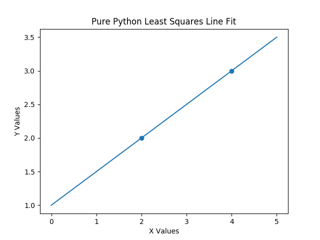
X = [2,4]
Y = [2,3]
plt.scatter(X,Y)

coefs = la.least_squares(X, Y)
la.print_matrix(coefs)

XLS = [0,1,2,3,4,5]
XLST = la.transpose(XLS)
XLST1 = la.insert_at_nth_column_of_matrix(1,XLST,1)
YLS = la.matrix_multiply(XLST1, coefs)

plt.plot(XLS, YLS)
plt.xlabel('X Values')
plt.ylabel('Y Values')
plt.title('Pure Python Least Squares Line Fit')
plt.show()

Wait! That’s just two points. You don’t even need least squares to do this one. That’s right. But it should work for this too – correct? Let’s walk through this code and then look at the output. Block 1 does imports. Block 2 looks at the data that we will use for fitting the model using a scatter plot. Block 3 does the actual fit of the data and prints the resulting coefficients for the model. Block 4 conditions some input data to the correct format and then front multiplies that input data onto the coefficients that were just found to predict additional results. Block 5 plots what we expected, which is a perfect fit, because our input data was in the column space of our output data. Figure 1 shows our plot.

Now, let’s produce some fake data that necessitates using a least squares approach. If you carefully observe this fake data, you will notice that I have sought to exactly balance out the errors for all data pairs. 

import LinearAlgebraPurePython as la 
import matplotlib.pyplot as plt

X = [2,3,4,2,3,4]
Y = [1.8,2.3,2.8,2.2,2.7,3.2]
plt.scatter(X,Y)

coefs = la.least_squares(X, Y)
la.print_matrix(coefs)

XLS = [0,1,2,3,4,5]
XLST = la.transpose(XLS)
XLST1 = la.insert_at_nth_column_of_matrix(1,XLST,1)
YLS = la.matrix_multiply(XLST1, coefs)

# print(YLS)
plt.plot(XLS, YLS)
plt.xlabel('X Values')
plt.ylabel('Y Values')
plt.title('Pure Python Least Squares Fake Noisy Data Fit')
plt.show()

The block structure is just like the block structure of the previous code, but we’ve artificially induced variations in the output data that should result in our least squares best fit line model passing perfectly between our data points. The output is shown in figure 2 below. 

OK. That worked, but will it work for more than one set of inputs? Let’s examine that using the next code block below. 

import LinearAlgebraPurePython as la 
import matplotlib.pyplot as plt
from mpl_toolkits.mplot3d import Axes3D
import sys

X = [[2,3,4,2,3,4],[1,2,3,1,2,3]]
Y = [1.8,2.3,2.8,2.2,2.7,3.2]
fig = plt.figure()
ax = plt.axes(projection='3d')

ax.scatter3D(X[0], X[1], Y)
ax.set_xlabel('X1 Values')
ax.set_ylabel('X2 Values')
ax.set_zlabel('Y Values')
ax.set_title('Pure Python Least Squares Two Inputs Data Fit')

coefs = la.least_squares(X, Y)
la.print_matrix(coefs)

XLS = [[1,1.5,2,2.5,3,3.5,4],[0,0.5,1,1.5,2,2.5,3]]
XLST = la.transpose(XLS)
XLST1 = la.insert_at_nth_column_of_matrix(1,XLST,len(XLST[0]))
YLS = la.matrix_multiply(XLST1, coefs)
YLST = la.transpose(YLS)

ax.plot3D(XLS[0], XLS[1], YLST[0])
plt.show()

The block structure follows the same structure as before, but, we are using two sets of input data now. Let’s look at the 3D output for this toy example in figure 3 below, which uses fake and well balanced output data for easy visualization of the least squares fitting concept. 

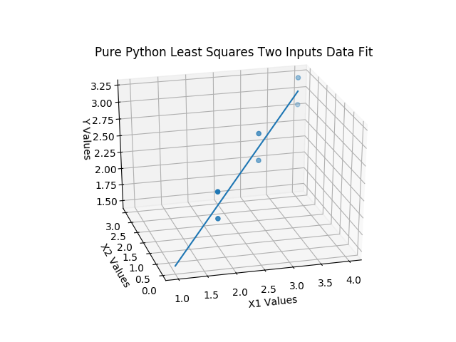
I really hope that you will clone the repo to at least play with this example, so that you can rotate the graph above to different viewing angles real time and see the fit from different angles. 

NOW FOR SOME REALISTIC DATA

Our realistic data set was obtained from HERE. Thanks! This file is in the repo for this post and is named LeastSquaresPractice_4.py.

The data has some inputs in text format. We have not yet covered encoding text data, but please feel free to explore the two functions included in the text block below that does that encoding very simply. We will cover one hot encoding in a future post in detail. Once we encode each text element to have it’s own column, where a “1” only occurs when the text element occurs for a record, and it has “0’s” everywhere else. For the number “n” of related encoded columns, we always have “n-1” columns, and the case where the two elements we use are both “0” is the case where the n^th element would exist. If we used the n^th column, we’d create a linear dependency (colinearity), and then our columns for the encoded variables would not be orthogonal as discussed in the previous post. We will cover linear dependency soon too.

We also haven’t talked about pandas yet. At this point, I’d encourage you to see what we are using it for below and make good use of those few steps. We’ll cover pandas in detail in future posts.

Also, the train_test_split is a method from the sklearn modules to use most of our data for training and some for testing. In testing, we compare our predictions from the model that was fit to the actual outputs in the test set to determine how well our model is predicting. We’ll cover more on training and testing techniques further in future posts also.

Again, all this code is in the repo.

import LinearAlgebraPurePython as la 
import pandas as pd
import numpy as np
from sklearn.preprocessing import OneHotEncoder
import sys


# Importing the dataset
df = pd.read_csv('50_Startups.csv')

# Segregating the data set
X = df.iloc[:, :-1].values
Y = df.iloc[:, 4].values

# Functions to help encode text / categorical data
def get_one_hot_encoding_for_one_column(X, i):
    col = X[:,i]
    labels = np.unique(col)
    ohe = OneHotEncoder(categories=[labels])
            
    return ohe

def apply_one_hot_encoder_on_matrix(ohe, X, i):
    col = X[:,i]
    tmp = ohe.fit_transform(col.reshape(-1, 1)).toarray()
    X = np.concatenate((X[:,:i], tmp[:,1:], X[:,i+1:]), axis=1)
    
    return X

# Use the two functions just defined above to encode cities
ohe = get_one_hot_encoding_for_one_column(X, 3)
X = apply_one_hot_encoder_on_matrix(ohe, X, 3)

# Splitting the dataset into the Training set and Test set
from sklearn.model_selection import train_test_split
X_train, X_test, Y_train, Y_test = train_test_split(
    X, Y, test_size = 0.2, random_state = 0)

# Convert Data to Pure Python Format
X_train = np.ndarray.tolist(X_train)
Y_train = np.ndarray.tolist(Y_train)
X_test = np.ndarray.tolist(X_test)
Y_test = np.ndarray.tolist(Y_test)

# Solve for the Least Squares Fit
coefs = la.least_squares(X_train, Y_train)
print('Pure Coefficients:')
la.print_matrix(coefs)
print()

# Print the output data
XLS1 = la.insert_at_nth_column_of_matrix(1,X_test,len(X_test[0]))
YLS = la.matrix_multiply(XLS1, coefs)
YLST = la.transpose(YLS)
print('PurePredictions:\n', YLST, '\n')

# Data produced from sklearn least squares model
SKLearnData = [103015.20159796, 132582.27760816, 132447.73845175, 
               71976.09851258, 178537.48221056, 116161.24230165, 
               67851.69209676, 98791.73374687, 113969.43533013, 
               167921.06569551]

# Print comparison of Pure and sklearn routines
print('Delta Between SKLearnPredictions and Pure Predictions:')
for i in range(len(SKLearnData)):
    delta = round(SKLearnData[i],6) - round(YLST[0][i],6)
    print('\tDelta for outputs {} is {}'.format(i, delta))

At this point, I will allow the comments in the code above to explain what each block of code does. Let’s look at the output from the above block of code. 

Pure Coefficients:
   [-959.284]
   [699.369]
   [0.773]
   [0.033]
   [0.037]
   [42554.168]

PurePredictions:
 [103015.20159796177, 132582.27760815577, 132447.73845174487, 
  71976.0985125791, 178537.48221055063, 116161.24230165093, 
  67851.69209675638, 98791.73374687451, 113969.4353301244, 
  167921.06569550425] 

Delta Between SKLearnPredictions and Pure Predictions:
    Delta for outputs 0 is 0.0
    Delta for outputs 1 is 0.0
    Delta for outputs 2 is 0.0
    Delta for outputs 3 is 0.0
    Delta for outputs 4 is 0.0
    Delta for outputs 5 is 0.0
    Delta for outputs 6 is 0.0
    Delta for outputs 7 is 0.0
    Delta for outputs 8 is 0.0
    Delta for outputs 9 is 0.0

It all looks good.

There’s one other practice file called LeastSquaresPractice_5.py that imports preconditioned versions of the data from conditioned_data.py. Both of these files are in the repo. The output’s the same. Check out the operation if you like. 

Using SKLearn For The Predictions

As you’ve seen above, we were comparing our results to predictions from the sklearn module. While we will cover many numpy, scipy and sklearn modules in future posts, it’s worth covering the basics of how we’d use the LinearRegression class from sklearn, and to cover that, we’ll go over the code below that was run to produce predictions to compare with our pure python module. The code below is stored in the repo for this post, and it’s name is LeastSquaresPractice_Using_SKLearn.py.

from sklearn.linear_model import LinearRegression
import pandas as pd
import numpy as np
from sklearn.preprocessing import OneHotEncoder
import sys

# Importing the dataset
df = pd.read_csv('50_Startups.csv')

# Segregating the data set
X = df.iloc[:, :-1].values
Y = df.iloc[:, 4].values

# Functions to help encode text / categorical data
def get_one_hot_encoding_for_one_column(X, i):
    col = X[:, i]
    labels = np.unique(col)
    ohe = OneHotEncoder(categories=[labels])

    return ohe

def apply_one_hot_encoder_on_matrix(ohe, X, i):
    col = X[:, i]
    tmp = ohe.fit_transform(col.reshape(-1, 1)).toarray()
    X = np.concatenate((X[:, :i], tmp[:, 1:], X[:, i+1:]), axis=1)

    return X

# Use the two functions just defined above to encode cities
ohe = get_one_hot_encoding_for_one_column(X, 3)
X = apply_one_hot_encoder_on_matrix(ohe, X, 3)

# Splitting the dataset into the Training set and Test set
from sklearn.model_selection import train_test_split
X_train, X_test, Y_train, Y_test = train_test_split(
    X, Y, test_size=0.2, random_state=0)

# Solve for the Least Squares Fit
lin_reg_model = LinearRegression()
lin_reg_model.fit(X_train, Y_train)
skl_predictions = lin_reg_model.predict(X_test)
print(skl_predictions)

# Data produced from sklearn least squares model
SKLearnData = [103015.20159796, 132582.27760816, 132447.73845175,
               71976.09851258, 178537.48221056, 116161.24230165,
               67851.69209676, 98791.73374687, 113969.43533013,
               167921.06569551]

The code blocks are much like those that were explained above for LeastSquaresPractice_4.py, but it’s a little shorter. Let’s cover the differences. In the first code block, we are not importing our pure python tools. Instead, we are importing the LinearRegression class from the sklearn.linear_model module. Then, like before, we use pandas features to get the data into a dataframe and convert that into numpy versions of our X and Y data. We define our encoding functions and then apply them to our X data as needed to turn our text based input data into 1’s and 0’s. We then split our X and Y data into training and test sets as before. We then fit the model using the training data and make predictions with our test data. We then used the test data to compare the pure python least squares tools to sklearn’s linear regression tool that used least squares, which, as you saw previously, matched to reasonable tolerances.

Closing

Where do we go from here? Next is fitting polynomials using our least squares routine. We’ll also create a class for our new least squares machine to better mimic the good operational nature of the sklearn version of least squares regression. We’ll then learn how to use this to fit curved surfaces, which has some great applications on the boundary between machine learning and system modeling and other cool/weird stuff. I’ll try to get those posts out ASAP.

Until next time …